Gravitational Lensing Example: CNN Embedding + Flow Matching#
![]()
This notebook demonstrates a Simulation-Based Inference (SBI) workflow for a Strong Lensing task.
Conceptual Overview#
We aim to infer the parameters \(\theta\) of a lensing system (e.g., lens mass, shear) given an observed image \(x\).
Strategy:
Compression (VAE): We use a Variational Autoencoder (VAE) to compress the high-dimensional conditioning data (32x32 images) into a lower-dimensional latent representation.
Inference (Flow Matching): We condition our inference model (a Flux1 Flow Matching model) on this latent representation.
The encoder is trained end-to-end with the flow matching model to optimize the inference objective.
Configuration & Data Dimensions#
We use the configuration from config_1a.yaml.
Data Dimensions#
Observation (\(\\theta\)): The target of inference. It has 2 features (parameters) and 1 channel.
Conditioning (\(x\)): Lensing images. 32x32 pixels with 1 channel.
Processing Pipeline#
The conditioning images go through several transformation steps before entering the inference model:
VAE Encoder: The 32x32x1 image is processed by the VAE encoder, which outputs a latent feature map of shape 8x8x16.
Patchification: We apply standard Vision Transformer (ViT) patchification with 2x2 patches.
Spatial dimension reduces by factor of 2: \(8 \to 4\).
Channel dimension increases by factor of \(2 \times 2 = 4\): \(16 \to 64\).
Resulting shape: 4x4x64.
Reshaping: For the Transformer, we flatten the spatial dimensions.
\(4 \times 4 = 16\) tokens.
Each token has size 64.
Resulting array: 16x64.
The pipeline handles the initialization of condition IDs to represent the patched structure of the image.
1. Setup and Imports#
First, we set up the environment and import necessary libraries.
# Check if running on Colab and install dependencies if needed
try:
    import google.colab
    colab = True
except ImportError:
    colab = False

if colab:
    # Install required packages and clone the repository
    !uv pip install --quiet "gensbi[cuda12,examples]"
    !git clone --depth 1 https://github.com/aurelio-amerio/GenSBI-examples
    %cd GenSBI-examples/examples/sbi-benchmarks/lensing
import os

if os.environ.get("JAX_PLATFORMS") is None:
    # os.environ["JAX_PLATFORMS"] = "cpu"
    os.environ["XLA_PYTHON_CLIENT_MEM_FRACTION"] = ".90"  # use 90% of GPU memory
    os.environ["JAX_PLATFORMS"] = "cuda"  # change to 'cpu' if no GPU is available

import gensbi

# base libraries
import jax
from jax import Array
from jax import numpy as jnp
import numpy as np
from flax import nnx

from tqdm import tqdm
import gc

# data loading
import grain
from datasets import load_dataset
import yaml

# plotting
import matplotlib.pyplot as plt

# gensbi
from gensbi.recipes import ConditionalPipeline
from gensbi.core import FlowMatchingMethod
from gensbi.recipes.flux1 import parse_flux1_params, parse_training_config
from gensbi.recipes.utils import patchify_2d

from gensbi.experimental.models.autoencoders import AutoEncoder2D, AutoEncoderParams
from gensbi.experimental.recipes.vae_pipeline import parse_autoencoder_params
from gensbi.models import Flux1Params, Flux1

from gensbi.utils.plotting import plot_marginals

from gensbi.diagnostics import LC2ST, plot_lc2st
from gensbi.diagnostics import run_sbc, sbc_rank_plot
from gensbi.diagnostics import run_tarp, plot_tarp

from gensbi_examples.tasks import GravitationalLensing

config_path = "./config/config_1a.yaml"
2. Helper Functions and Classes#
def normalize(batch, mean, std):
    mean = jnp.asarray(mean, dtype=batch.dtype)
    std = jnp.asarray(std, dtype=batch.dtype)
    return (batch - mean) / std


def unnormalize(batch, mean, std):
    mean = jnp.asarray(mean, dtype=batch.dtype)
    std = jnp.asarray(std, dtype=batch.dtype)
    return batch * std + mean


class LensingModel(nnx.Module):
    """
    A combined model that first encodes the conditioning data (images) using a VAE,
    and then passes the latent embedding to the SBI model (Flux).
    """
    def __init__(self, vae, sbi_model):
        self.vae = vae
        self.sbi_model = sbi_model

    def __call__(
        self,
        t: Array,
        obs: Array,
        obs_ids: Array,
        cond: Array,
        cond_ids: Array,
        conditioned: bool | Array = True,
        guidance: Array | None = None,
        encoder_key=None,
    ):

        # first we encode the conditioning data
        cond_latent = self.vae.encode(cond, encoder_key)
        # patchify the cond_latent for the transformer
        cond_latent = patchify_2d(cond_latent)

        # then we pass to the sbi model
        return self.sbi_model(
            t=t,
            obs=obs,
            obs_ids=obs_ids,
            cond=cond_latent,
            cond_ids=cond_ids,
            conditioned=conditioned,
            guidance=guidance,
        )
3. Data Loading#
We load the Lensing dataset.
dim_obs = 2
ch_obs = 1

task = GravitationalLensing()

df_train = task.df_train
df_val = task.df_val
df_test = task.df_test

xs_mean = jnp.array([-1.1874731e-05], dtype=jnp.bfloat16).reshape(1, 1, 1)
thetas_mean = jnp.array([0.5996428, 0.15998043], dtype=jnp.bfloat16).reshape(1, 2)

xs_std = jnp.array([1.0440514], dtype=jnp.bfloat16).reshape(1, 1, 1)
thetas_std = jnp.array([0.2886958, 0.08657552], dtype=jnp.bfloat16).reshape(1, 2)
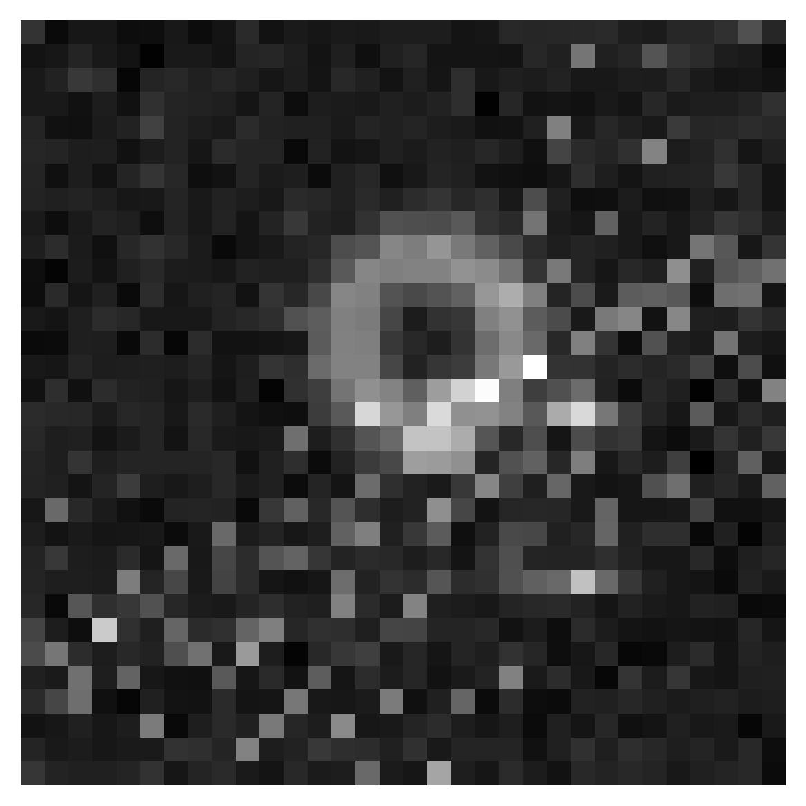
# plot a sample
x_o = df_test["xs"][0][None, ...]
x_o = normalize(jnp.array(x_o, dtype=jnp.bfloat16), xs_mean, xs_std)

theta_true = df_test["thetas"][0]  # already unnormalized
plt.imshow(x_o[0], cmap="gray")
plt.axis("off")
plt.savefig("img/lensing.png", bbox_inches="tight", dpi=300)
plt.show()
4. Model Initialization#
params_dict = parse_autoencoder_params(config_path)

ae_params = AutoEncoderParams(
    rngs=nnx.Rngs(0),
    **params_dict,
)

# define the vae model
vae_model = AutoEncoder2D(ae_params)

# for the sake of the NPE, we delete the decoder model as it is not needed
vae_model.Decoder1D = None
# run the garbage collector to free up memory
gc.collect()

# now we define the NPE pipeline
# get the latent dimensions from the autoencoder
latent_dim1 = vae_model.latent_shape[1]
latent_dim2 = vae_model.latent_shape[2]

# After 2x2 patchification, dimensions are halved
dim_cond_latent = (latent_dim1 // 2) * (latent_dim2 // 2)
# Channels are multiplied by 4 (2x2)
ch_cond_latent = vae_model.latent_shape[3] * 4

print(f"Original Latent Shape: {vae_model.latent_shape}")
print(f"Conditioning Transformer Input: {dim_cond_latent} tokens of size {ch_cond_latent}")

params_dict_flux = parse_flux1_params(config_path)
assert (
    params_dict_flux["context_in_dim"] == ch_cond_latent
), "Context dimension mismatch, got {} expected {}".format(
    params_dict_flux["context_in_dim"], ch_cond_latent
)

params_flux = Flux1Params(
    rngs=nnx.Rngs(0),
    dim_obs=dim_obs,
    dim_cond=dim_cond_latent,
    **params_dict_flux,
)

model_sbi = Flux1(params_flux)

model = LensingModel(vae_model, model_sbi)
5. Pipeline Setup and Restoration#
training_config = parse_training_config(config_path)

with open(config_path, "r") as f:
    config = yaml.safe_load(f)
    batch_size = config["training"]["batch_size"]
    nsteps = config["training"]["nsteps"]
    multistep = config["training"]["multistep"]
    experiment = config["training"]["experiment_id"]

def split_data(batch):
    obs = jnp.array(batch["thetas"], dtype=jnp.bfloat16)
    obs = normalize(obs, thetas_mean, thetas_std)
    obs = obs.reshape(obs.shape[0], dim_obs, ch_obs)
    cond = jnp.array(batch["xs"], dtype=jnp.bfloat16)
    cond = normalize(cond, xs_mean, xs_std)
    cond = cond[..., None]
    return obs, cond

train_dataset_npe = (
    grain.MapDataset.source(df_train).shuffle(42).repeat().to_iter_dataset()
)

performance_config = grain.experimental.pick_performance_config(
    ds=train_dataset_npe,
    ram_budget_mb=1024 * 8,
    max_workers=None,
    max_buffer_size=None,
)

train_dataset_npe = (
    train_dataset_npe.batch(batch_size)
    .map(split_data)
    .mp_prefetch(performance_config.multiprocessing_options)
)

val_dataset_npe = (
    grain.MapDataset.source(df_val)
    .shuffle(42)
    .repeat()
    .to_iter_dataset()
    .batch(256)
    .map(split_data)
)

# Set checkpoint directory
current_dir = os.getcwd()
checkpoint_dir = os.path.join(current_dir, "checkpoints")
training_config["checkpoint_dir"] = checkpoint_dir

pipeline_latent = ConditionalPipeline(
    model,
    train_dataset_npe,
    val_dataset_npe,
    dim_obs=dim_obs,
    dim_cond=(
        latent_dim1,
        latent_dim2,
    ),  # we are workin in the latent space of the vae
    ch_obs=ch_obs,
    ch_cond=ch_cond_latent,  # conditioning is now in the latent space
    method = FlowMatchingMethod(), # use flow matching
    training_config=training_config,
    id_embedding_strategy=("absolute", "rope2d"),
)

print("Restoring model...")
pipeline_latent.restore_model()
print("Done!")
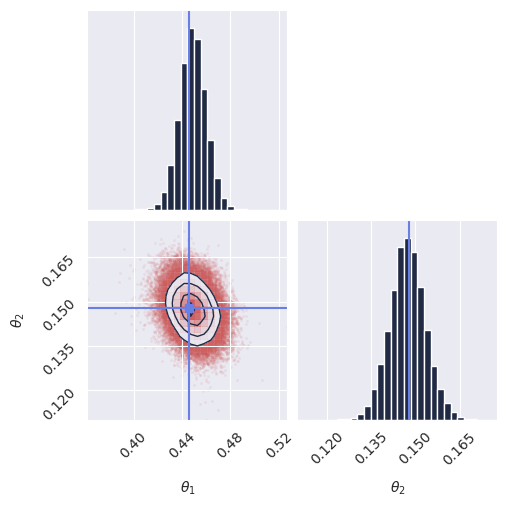
6. Inference and Visualization#
We generate samples and visualize the posterior for a test observation.
x_o = df_test["xs"][0][None, ...]
x_o = normalize(jnp.array(x_o, dtype=jnp.bfloat16), xs_mean, xs_std)
x_o = x_o[..., None]

theta_true = df_test["thetas"][0]  # already unnormalized

print("Sampling 100,000 samples...")
samples = pipeline_latent.sample_batched(
    nnx.Rngs(0).sample(),
    x_o,
    100_000,
    chunk_size=10_000,
    encoder_key=jax.random.PRNGKey(1234),
)

res = samples[:, 0, :, 0]  # shape (num_samples, 1, 2, 1) -> (num_samples, 2)
# unnormalize the results for plotting
res_unnorm = unnormalize(res, thetas_mean, thetas_std)

plot_marginals(res_unnorm, true_param=theta_true, gridsize=30)
plt.title(f"Lensing Samples (Exp {experiment})")
# plt.savefig(f"imgs/lensing_samples_conf{experiment}.png", dpi=100, bbox_inches="tight")
plt.show()
7. Diagnostics#
You should run several diagnostics to validate the quality of the posterior estimation.
We leave as an excercise the implementation of these diagnostics (or take a look at the training script: train-lensing.py).
Below are the results of the diagnostics for the lensing example.
Note:
Running these tests is slow, and requires a GPU.
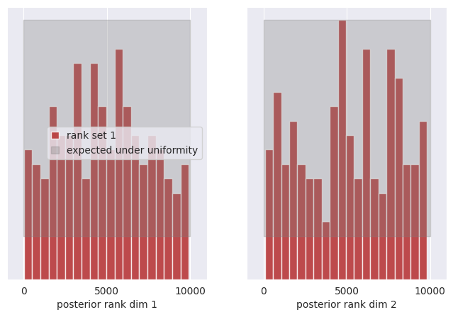
SBC:
Marginal coverage:
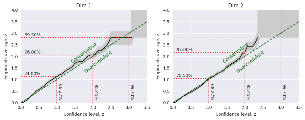
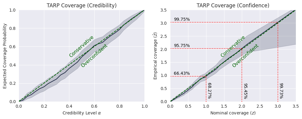
TARP:
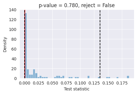
L-C2ST:
Conclusions#
The SBC test tells us that the posterior for the first dimension is reasonable, while the second dimension is slightly skewed.
The marginal coverage test tells us that the the posterior for the first dimension is slightly underconfident while the second dimension is slightly overconfident.
The TARP test tells us that the posterior is overall well-calibrated, but the model is slightly overconfident in the region around the peak of the distribution (\(\alpha\)<0.6).
The L-C2ST test tells us that a local classifier cannot distinguish samples drawan from the true joint distributions, and samples drawn from the model, meaning that we can’t reject the hypothesis that the model is well calibrated.
Final remark: The model in this example has been trained in a “fast” configuration, as an example, and can be further refined by optimizing the model parameters and training configuration.