15-minute quick start

Welcome to GenSBI! This page is a quick guide to get you started with installation and basic usage.

Installation

GenSBI is in early development. To install, clone the repository and install dependencies:

pip install gensbi

If a GPU is available, it is advisable to install the cuda version of the package:

pip install gensbi[cuda12]

Requirements

• Python 3.11+

• JAX

• Flax

• (See pyproject.toml for full requirements)

Basic Usage

To get started fast, use the provided recipes.

Note

The example below is a minimal script designed for copy-pasting by experienced users. If you want a step-by-step educational walkthrough that explains the concepts, please see the My First Model Tutorial.

Here is a minimal example of setting up a flow-based conditional inference pipeline using Flux1.

This example covers:

1. Data Generation: Creating synthetic data for a simple linear problem.

2. Model Configuration: Setting up the Flux1 parameters.

3. Pipeline Creation: Initializing the Flux1FlowPipeline which handles training and sampling.

4. Training: Running the training loop.

5. Inference: Sampling from the posterior given new observation.

The code below is a complete, runnable script:

# %% Imports
import os

# Set JAX backend (use 'cuda' for GPU, 'cpu' otherwise)
# os.environ["JAX_PLATFORMS"] = "cuda"

import grain
import numpy as np
import jax
from jax import numpy as jnp
from numpyro import distributions as dist
from flax import nnx

from gensbi.recipes import Flux1FlowPipeline
from gensbi.models import Flux1, Flux1Params

from gensbi.utils.plotting import plot_marginals
import matplotlib.pyplot as plt


# %%

theta_prior = dist.Uniform(
    low=jnp.array([-2.0, -2.0, -2.0]), high=jnp.array([2.0, 2.0, 2.0])
)

dim_obs = 3
dim_cond = 3
dim_joint = dim_obs + dim_cond


# %%
def simulator(key, nsamples):
    theta_key, sample_key = jax.random.split(key, 2)
    thetas = theta_prior.sample(theta_key, (nsamples,))

    xs = thetas + 1 + jax.random.normal(sample_key, thetas.shape) * 0.1

    thetas = thetas[..., None]
    xs = xs[..., None]

    # when making a dataset for the joint pipeline, thetas need to come first
    data = jnp.concatenate([thetas, xs], axis=1)

    return data


# %% Define your training and validation datasets.
# We generate a training dataset and a validation dataset using the simulator.
# The simulator is a simple function that generates parameters (theta) and data (x).
# In this example, we use a simple Gaussian simulator.
train_data = simulator(jax.random.PRNGKey(0), 100_000)
val_data = simulator(jax.random.PRNGKey(1), 2000)


# %% Normalize the dataset
# It is important to normalize the data to have zero mean and unit variance.
# This helps the model training process.
means = jnp.mean(train_data, axis=0)
stds = jnp.std(train_data, axis=0)


def normalize(data, means, stds):
    return (data - means) / stds


def unnormalize(data, means, stds):
    return data * stds + means


# %% Prepare the data for the pipeline
# The pipeline expects the data to be split into observations and conditions.
# We also apply normalization at this stage.
def split_obs_cond(data):
    data = normalize(data, means, stds)
    return (
        data[:, :dim_obs],
        data[:, dim_obs:],
    )  # assuming first dim_obs are obs, last dim_cond are cond


# %%

# %% Create the input pipeline using Grain
# We use Grain to create an efficient input pipeline.
# This involves shuffling, repeating for multiple epochs, and batching the data.
# We also map the split_obs_cond function to prepare the data for the model.
batch_size = 256

train_dataset_grain = (
    grain.MapDataset.source(np.array(train_data))
    .shuffle(42)
    .repeat()
    .to_iter_dataset()
    .batch(batch_size)
    .map(split_obs_cond)
    # .mp_prefetch() # Uncomment if you want to use multiprocessing prefetching
)

val_dataset_grain = (
    grain.MapDataset.source(np.array(val_data))
    .shuffle(42)
    .repeat()
    .to_iter_dataset()
    .batch(batch_size)
    .map(split_obs_cond)
    # .mp_prefetch() # Uncomment if you want to use multiprocessing prefetching
)

# %% Define your model
# specific model parameters are defined here.
# For Flux1, we need to specify dimensions, embedding strategies, and other architecture details.
params = Flux1Params(
    in_channels=1,
    vec_in_dim=None,
    context_in_dim=1,
    mlp_ratio=3,
    num_heads=2,
    depth=4,
    depth_single_blocks=8,
    axes_dim=[
        10,
    ],
    qkv_bias=True,
    dim_obs=dim_obs,
    dim_cond=dim_cond,
    theta=10 * dim_joint,
    id_embedding_strategy=("absolute", "absolute"),
    rngs=nnx.Rngs(default=42),
    param_dtype=jnp.float32,
)


# %% Instantiate the pipeline
# The Flux1FlowPipeline handles the training loop and sampling.
# We configure it with the model parameters, datasets, dimensions using a default training configuration.
training_config = Flux1FlowPipeline.get_default_training_config()
training_config["nsteps"] = 10000

pipeline = Flux1FlowPipeline(
    train_dataset_grain,
    val_dataset_grain,
    dim_obs,
    dim_cond,
    params=params,
    training_config=training_config,
)

# %% Train the model
# We create a random key for training and start the training process.
rngs = nnx.Rngs(42)
pipeline.train(
    rngs, save_model=False
)  # if you want to save the model, set save_model=True

# %% Sample from the posterior
# To generate samples, we first need an observation (and its corresponding condition).
# We generate a new sample from the simulator, normalize it, and extract the condition x_o.

new_sample = simulator(jax.random.PRNGKey(20), 1)
true_theta = new_sample[:, :dim_obs, :]  # extract observation from the joint sample

new_sample = normalize(new_sample, means, stds)
x_o = new_sample[:, dim_obs:, :]  # extract condition from the joint sample

# Then we invoke the pipeline's sample method.
samples = pipeline.sample(rngs.sample(), x_o, nsamples=100_000)
# Finally, we unnormalize the samples to get them back to the original scale.
samples = unnormalize(samples, means[:dim_obs], stds[:dim_obs])

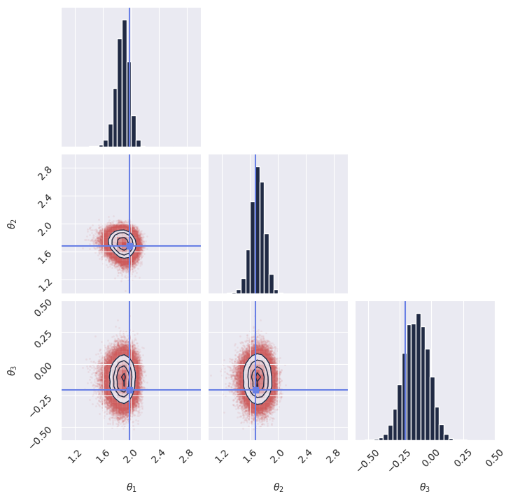
# %% Plot the samples
# We verify the model's performance by plotting the marginal distributions of the generated samples
# against the true parameters.
plot_marginals(
    np.array(samples[..., 0]),
    gridsize=30,
    true_param=np.array(true_theta[0, :, 0]),
    range=[(1, 3), (1, 3), (-0.6, 0.5)],
)
plt.savefig("flux1_flow_pipeline_marginals.png", dpi=100, bbox_inches="tight")
plt.show()

Note

If you plan on using multiprocessing prefetching, ensure that your script is wrapped in a if __name__ == "__main__": guard. See https://docs.python.org/3/library/multiprocessing.html

See the full example notebook my_first_model for a more detailed walkthrough, and the Examples page for practical demonstrations on common SBI benchmarks.

Citing GenSBI

If you use this library, please consider citing this work and the original methodology papers, see references.

@misc{GenSBI,
  author       = {Amerio, Aurelio},
  title        = "{GenSBI: Generative models for Simulation-Based Inference}",
  year         = {2025}, 
  publisher    = {GitHub},
  journal      = {GitHub repository},
  howpublished = {\url{https://github.com/aurelio-amerio/GenSBI}}
}