Bernoulli GLM Flux1 Flow Example#

Notice: This notebook has been automatically generated. If you find any errors, please open an issue on the GenSBI-examples GitHub repository.

This notebook demonstrates conditional Flow Matching on the Bernoulli GLM task using JAX and Flax.

Table of Contents#

Section	Description
1. Introduction & Setup	Overview, environment, device, autoreload
2. Task & Data Preparation	Define task, visualize data, create datasets
3. Model Configuration & Definition	Load config, set parameters, instantiate model
4. Training	Train or restore model, manage checkpoints
5. Evaluation & Visualization	Visualize loss, sample posterior, compute log prob
6. Posterior Calibration Checks	Marginal coverage, TARP, SBC, L-C2ST

1. Introduction & Setup#

In this section, we introduce the problem, set up the computational environment, import required libraries, configure JAX for CPU or GPU usage, and enable autoreload for iterative development. Compatibility with Google Colab is also ensured.

# Check if running on Colab and install dependencies if needed
try:
    import google.colab
    colab = True
except ImportError:
    colab = False

if colab:
    # Install required packages and clone the repository
    !uv pip install --quiet "gensbi[cuda12] @ git+https://github.com/aurelio-amerio/GenSBI"
    !uv pip install --quiet "gensbi-examples @ git+https://github.com/aurelio-amerio/GenSBI-examples"
    !git clone --depth 1 https://github.com/aurelio-amerio/GenSBI-examples
    %cd GenSBI-examples/examples/sbi-benchmarks/bernoulli_glm/flow_flux

import os
# select device

os.environ["JAX_PLATFORMS"] = "cuda" 
# os.environ["JAX_PLATFORMS"] = "cpu" 

2. Task & Data Preparation#

In this section, we define the Bernoulli GLM task, visualize reference samples, and create the training and validation datasets required for model learning. Batch size and sample count are set for reproducibility and performance.

restore_model=True
train_model=False

import orbax.checkpoint as ocp
# get the current notebook path
notebook_path = os.getcwd()
checkpoint_dir = os.path.join(notebook_path, "checkpoints")
os.makedirs(checkpoint_dir, exist_ok=True)

import matplotlib.pyplot as plt
import jax
import jax.numpy as jnp
from flax import nnx

from numpyro import distributions as dist
import numpy as np

from gensbi.utils.plotting import plot_marginals

from gensbi_examples.tasks import get_task
task = get_task("bernoulli_glm", kind="conditional", use_multiprocessing=False)

# reference posterior for an observation
obs, reference_samples = task.get_reference(num_observation=8)

# plot the 2D posterior 
plot_marginals(np.asarray(reference_samples, dtype=np.float32), gridsize=50, plot_levels=False, backend="seaborn")
plt.show()

# make a dataset
nsamples = int(1e5)

# Set batch size for training. Larger batch sizes help prevent overfitting, but are limited by available GPU memory.
batch_size = 4096
# Create training and validation datasets using the Bernoulli GLM task object.
train_dataset = task.get_train_dataset(batch_size)
val_dataset = task.get_val_dataset(batch_size)

# Create iterators for the training and validation datasets.
dataset_iter = iter(train_dataset)
val_dataset_iter = iter(val_dataset)

3. Model Configuration & Definition#

In this section, we load the model and optimizer configuration, set all relevant parameters, and instantiate the Flux1 model. Edge masks and marginalization functions are used for flexible inference and posterior estimation.

from gensbi.recipes import Flux1FlowPipeline

import yaml

# Path to the configuration file.
config_path = f"{notebook_path}/config/config_flow_flux.yaml"

# Extract dimensionality information from the task object.
dim_obs = task.dim_obs  # Number of parameters to infer
dim_cond = task.dim_cond    # Number of observed data dimensions

dim_joint = task.dim_joint  # Joint dimension (for model input)

pipeline = Flux1FlowPipeline.init_pipeline_from_config(
        train_dataset,
        val_dataset,
        dim_obs,
        dim_cond,
        config_path,
        checkpoint_dir,
    )

4. Training#

In this section, we train the model or restore a checkpoint.

# pipeline.train(nnx.Rngs(0), save_model=False)

pipeline.restore_model()

5. Evaluation & Visualization#

In this section, we evaluate the trained Simformer model by sampling from the posterior, and comparing results to reference data.

Section 5.1: Posterior Sampling#

In this section, we sample from the posterior distribution using the trained model and visualize the results. Posterior samples are generated for a selected observation and compared to reference samples to assess model accuracy.

# we want to do conditional inference. We need an observation for which we want to ocmpute the posterior
def get_samples(idx, nsamples=10_000, use_ema=False, key=None):
    observation, reference_samples = task.get_reference(idx)
    true_param = jnp.array(task.get_true_parameters(idx))

    if key is None:
        key = jax.random.PRNGKey(42)

    time_grid = jnp.linspace(0,1,100)

    samples = pipeline.sample(key, observation, nsamples, use_ema=use_ema, time_grid=time_grid)
    return samples, true_param, reference_samples

samples, true_param, reference_samples =  get_samples(8)

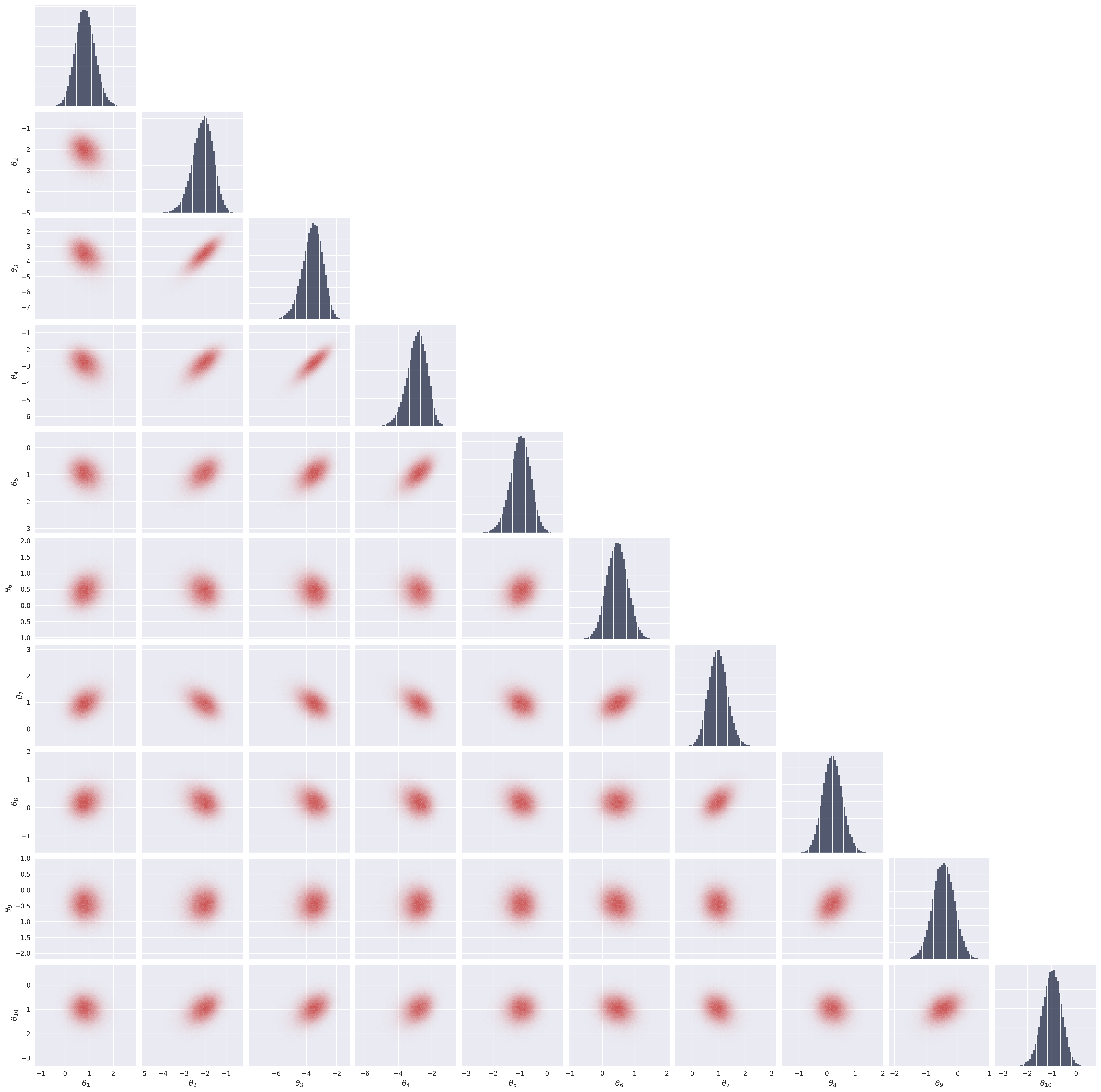
Section 5.2: Visualize Posterior Samples#

In this section, we plot the posterior samples as a 2D histogram to visualize the learned distribution and compare it to the ground truth.

from gensbi.utils.plotting import plot_marginals, plot_2d_dist_contour

plot_marginals(samples[-1,...,0], backend="seaborn", gridsize=50)
plt.show()

# alternatively use "corner" to plot containment levels too
# plot_marginals(samples[-1,...,0], backend="corner", gridsize=20)
# plt.show()

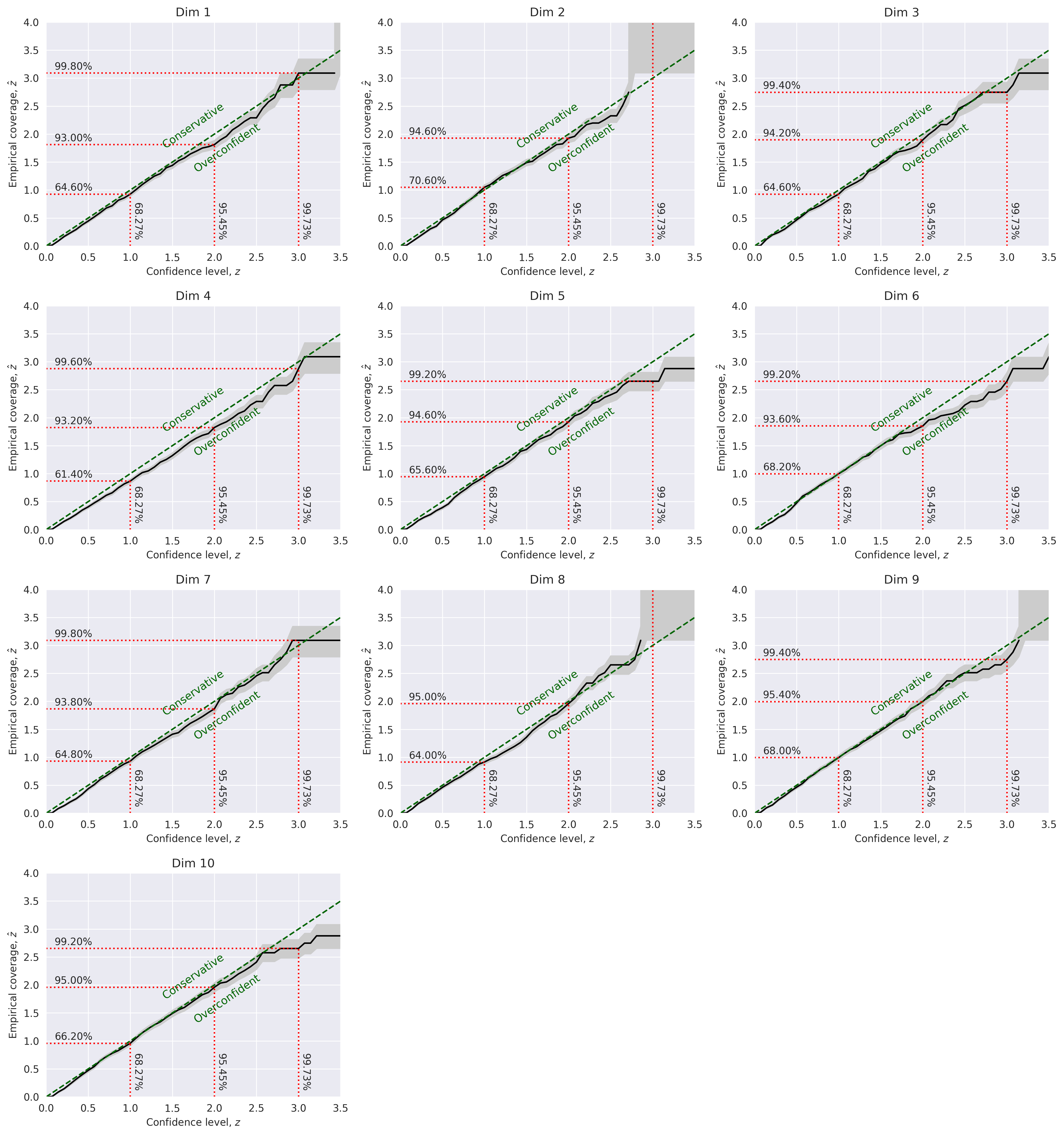
6. Posterior Calibration Checks#

We report here the results of the posterior calibration tests. As an excercise, you can implement the tests as in the Two Moons example and compare the results.

Average C2ST: 0.5594 ± 0.0143

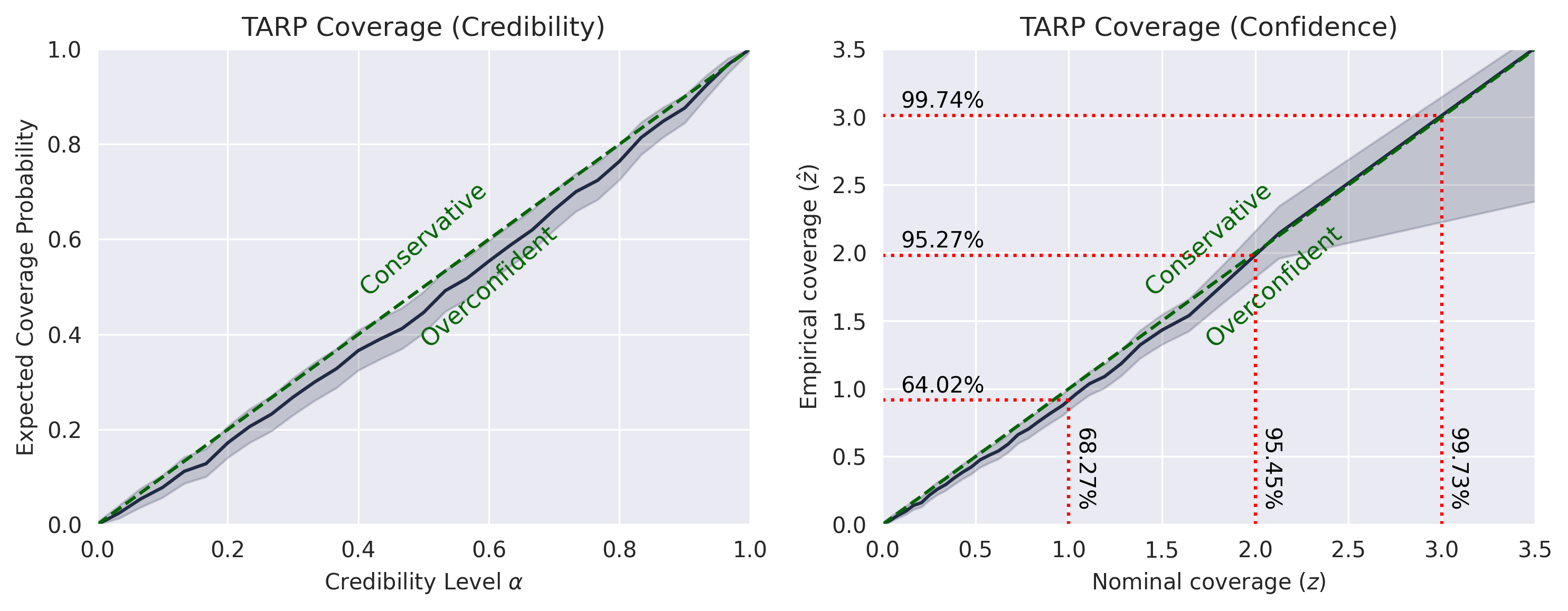
Marginal Coverage:

TARP:

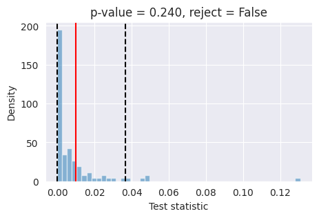
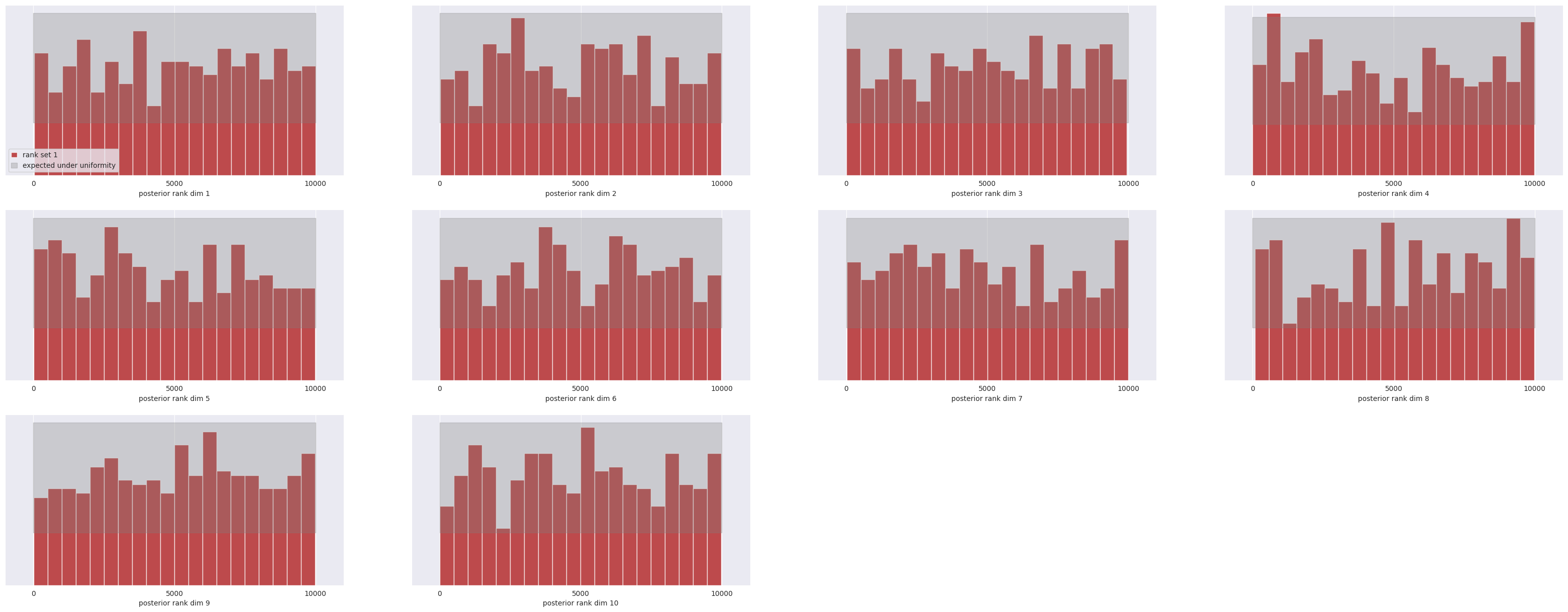
SBC

L-C2ST