Two Moons Flux1Joint Flow Matching Example

---

This notebook demonstrates conditional Flow Matching on the Two Moons task using JAX and Flax.

About Simulation-Based Inference (SBI): SBI refers to a class of methods for inferring parameters of complex models when the likelihood function is intractable, but simulation is possible. SBI algorithms learn to approximate the posterior distribution over parameters given observed data, enabling inference in scientific and engineering domains where traditional methods fail.

The Two Moons Dataset: The Two Moons dataset is a two-dimensional simulation-based inference benchmark designed to test an algorithm’s ability to handle complex posterior distributions. Its posterior is both bimodal (two distinct peaks) and locally crescent-shaped, making it a challenging task for inference algorithms. The primary purpose of this benchmark is to evaluate how well different methods can capture and represent multimodality and intricate structure in the posterior.

Purpose of This Notebook: This notebook trains and evaluates a Flux1Joint Flow Matching model on the Two Moons task. The goal is to assess the model’s ability to learn and represent a non-trivial posterior distribution with both global (bimodal) and local (crescent-shaped) complexity.

Table of Contents

Section	Description
1. Introduction & Setup	Overview, environment, device, autoreload
2. Task & Data Preparation	Define task, visualize data, create datasets
3. Model Configuration & Definition	Load config, set parameters, instantiate model
4. Training	Train or restore model, manage checkpoints
5. Evaluation & Visualization	Visualize loss, sample posterior, compute log prob
6. Posterior Calibration Checks	Marginal coverage, TARP, SBC, L-C2ST

---

1. Introduction & Setup

---

In this section, we introduce the problem, set up the computational environment, import required libraries, configure JAX for CPU or GPU usage, and enable autoreload for iterative development. Compatibility with Google Colab is also ensured.

# Check if running on Colab and install dependencies if needed
try:
    import google.colab
    colab = True
except ImportError:
    colab = False

if colab:
    # Install required packages and clone the repository
    !uv pip install --quiet "gensbi[cuda12, examples] @ git+https://github.com/aurelio-amerio/GenSBI"
    !git clone --depth 1 https://github.com/aurelio-amerio/GenSBI-examples
    %cd GenSBI-examples/examples/sbi-benchmarks/two_moons/flow_flux1joint

import os
# select device

os.environ["JAX_PLATFORMS"] = "cuda" 
# os.environ["JAX_PLATFORMS"] = "cpu" 

2. Task & Data Preparation

---

In this section, we define the Two Moons task, visualize reference samples, and create the training and validation datasets required for model learning. Batch size and sample count are set for reproducibility and performance.

restore_model=True
train_model=False

import orbax.checkpoint as ocp
# get the current notebook path
notebook_path = os.getcwd()
checkpoint_dir = os.path.join(notebook_path, "checkpoints")
os.makedirs(checkpoint_dir, exist_ok=True)

import matplotlib.pyplot as plt
import jax
import jax.numpy as jnp
from flax import nnx

from numpyro import distributions as dist
import numpy as np

from gensbi.utils.plotting import plot_marginals

from gensbi_examples.tasks import TwoMoons
task = TwoMoons(kind="joint")

# reference posterior for an observation
obs, reference_samples = task.get_reference(num_observation=8)

# plot the 2D posterior 
plot_marginals(np.asarray(reference_samples, dtype=np.float32), gridsize=50,range=[(-1,0),(0,1)], plot_levels=False, backend="seaborn")
plt.show()

# make a dataset
nsamples = int(1e5)

# Set batch size for training. Larger batch sizes help prevent overfitting, but are limited by available GPU memory.
batch_size = 4096
# Create training and validation datasets using the Two Moons task object.
train_dataset = task.get_train_dataset(batch_size)
val_dataset = task.get_val_dataset(batch_size)

# Create iterators for the training and validation datasets.
dataset_iter = iter(train_dataset)
val_dataset_iter = iter(val_dataset)

3. Model Configuration & Definition

---

In this section, we load the model and optimizer configuration, set all relevant parameters, and instantiate the Flux1Joint model. Edge masks and marginalization functions are used for flexible inference and posterior estimation.

from gensbi.recipes import Flux1JointFlowPipeline

import yaml

# Path to the Flux1Joint Flow Matching configuration file.
config_path = f"{notebook_path}/config/config_flow_flux1joint.yaml"

# Extract dimensionality information from the task object.
dim_obs = task.dim_obs  # Number of parameters to infer
dim_cond = task.dim_cond    # Number of observed data dimensions

dim_joint = dim_obs + dim_cond  # Joint dimension (for model input)

pipeline = Flux1JointFlowPipeline.init_pipeline_from_config(
        train_dataset,
        val_dataset,
        dim_obs,
        dim_cond,
        config_path,
        checkpoint_dir,
    )

4. Training

---

In this section, we train the Flow Matching model or restore a checkpoint.

# pipeline.train(nnx.Rngs(0), 5, save_model=False)

pipeline.restore_model()

5. Evaluation & Visualization

---

In this section, we evaluate the trained Simformer model by sampling from the posterior, and comparing results to reference data. We also compute and visualize the unnormalized log probability over a grid to assess model calibration and density estimation. These analyses provide insight into model performance and reliability.

Section 5.1: Posterior Sampling

---

In this section, we sample from the posterior distribution using the trained model and visualize the results. Posterior samples are generated for a selected observation and compared to reference samples to assess model accuracy.

# we want to do conditional inference. We need an observation for which we want to ocmpute the posterior
def get_samples(idx, nsamples=10_000, use_ema=False, key=None):
    observation, reference_samples = task.get_reference(idx)
    true_param = jnp.array(task.get_true_parameters(idx))

    if key is None:
        key = jax.random.PRNGKey(42)

    time_grid = jnp.linspace(0,1,100)

    samples = pipeline.sample(key, observation, nsamples, use_ema=use_ema, time_grid=time_grid)
    return samples, true_param, reference_samples

samples, true_param, reference_samples =  get_samples(8)

samples.shape # (100, 10000, 2)

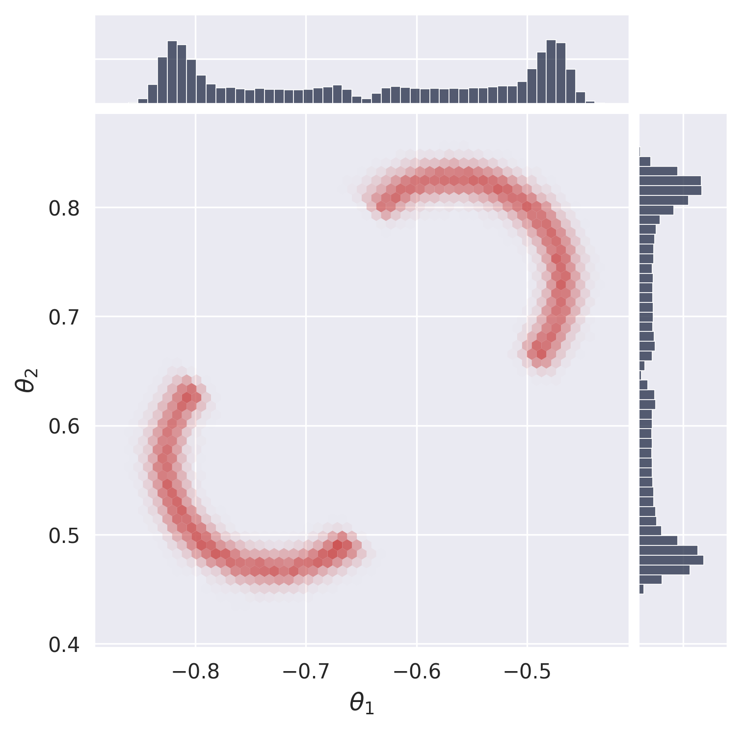
Section 5.2: Visualize Posterior Samples

---

In this section, we plot the posterior samples as a 2D histogram to visualize the learned distribution and compare it to the ground truth.

from gensbi.utils.plotting import plot_marginals, plot_2d_dist_contour

plot_marginals(samples[-1,...,0], plot_levels=False, backend="seaborn", gridsize=50, range =[(-1., 0), (0, 1.)])
plt.show()

# alternatively use "corner" to plot containment levels too
# plot_marginals(samples[-1,...,0], plot_levels=True, gridsize=30, range=[(-1., 0), (0, 1.)])
# plt.show()

5.3. Animations

---

In this section, we create and display animations of posterior samples and density contours over time. These visualizations illustrate the evolution of the learned distribution during the sampling process, providing dynamic insight into model behavior and convergence.

import imageio.v3 as imageio
import io
from tqdm import tqdm

# samples

images = []

for i in tqdm(range(len(samples))):
    fig, axes = plot_marginals(
        samples[i,...,0],
        plot_levels=False,
        gridsize=50,
        range=[(-1.0, 0), (0, 1.0)],
        backend="seaborn",
    )

    # manually set the ticks to make a prettier plot
   
    axes[0,0].set_ylim(0,6)
    axes[0,0].set_yticks([5])

    axes[1,1].set_xlim(0,6)
    axes[1,1].set_xticks([5])

    axes[1,1].text(0, 1.03, f"t = {(i+1)/len(samples):.2f}", transform=plt.gca().transAxes)

    buf = io.BytesIO()
    plt.savefig(buf, format="png", dpi=300)
    buf.seek(0)
    image = imageio.imread(buf)
    buf.close()
    if i == 0:
        images = []
    images.append(image)
    plt.close()

# repeat the last frame 10 times to make the gif pause at the end
images += [images[-1]] * 20

imageio.imwrite(
    'animated_plot_samples.gif', 
    images, 
    duration=5000/len(images), 
    loop=0  # 0 means loop indefinitely
)

6. Posterior Calibration Checks

import warnings
warnings.filterwarnings(
    "ignore", category=UserWarning, module="google.protobuf.runtime_version"
)

from gensbi.diagnostics import run_sbc, sbc_rank_plot
from gensbi.diagnostics import run_tarp, plot_tarp
from gensbi.diagnostics.marginal_coverage import compute_marginal_coverage, plot_marginal_coverage
from gensbi.diagnostics import LC2ST, plot_lc2st
import matplotlib.pyplot as plt
import jax.numpy as jnp
import numpy as np
import jax

num_calibration_samples = 200 #excercise: try 500, what changes?
num_posterior_samples = 1000 #excercise: try 10_000, what changes?

# Get test data
data = task.dataset["test"].with_format("jax")[:num_calibration_samples]
xs = jnp.asarray(data["xs"], dtype=jnp.bfloat16)
thetas = jnp.asarray(data["thetas"], dtype=jnp.bfloat16)

print(f"Sampling {num_posterior_samples} posterior samples for {num_calibration_samples} observations...")

# Generate posterior samples in batch
posterior_samples = pipeline.sample_batched(
    jax.random.PRNGKey(12345), xs, num_posterior_samples, use_ema=True
)

# Reshape for analysis
xs = xs.reshape((xs.shape[0], -1))
thetas = thetas.reshape((thetas.shape[0], -1))
posterior_samples = posterior_samples.reshape(
    (posterior_samples.shape[0], posterior_samples.shape[1], -1)
)

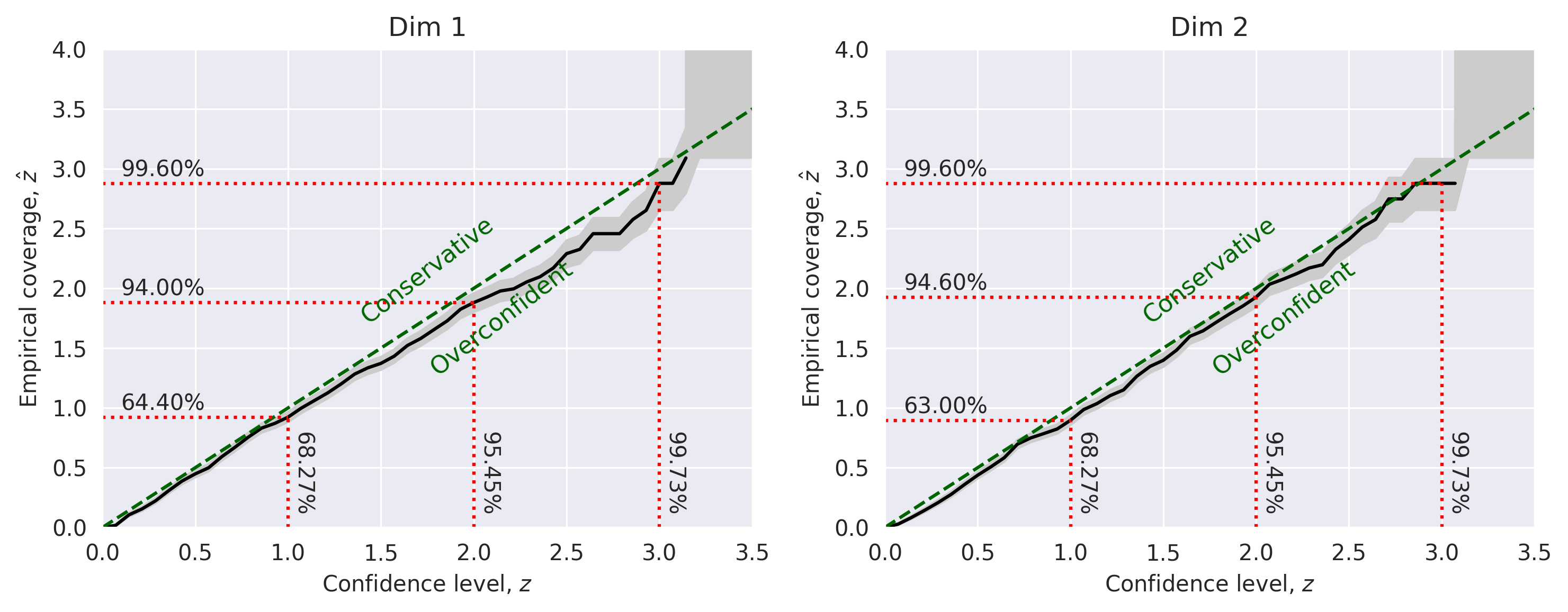
6.1. Marginal coverage

In this test, we compare the expected confidence level \(z\) with the empirical coverage level \(\hat{z}\) for each parameter.

alpha_marginal = compute_marginal_coverage(thetas, posterior_samples, method="histogram")
plot_marginal_coverage(alpha_marginal)
plt.show()

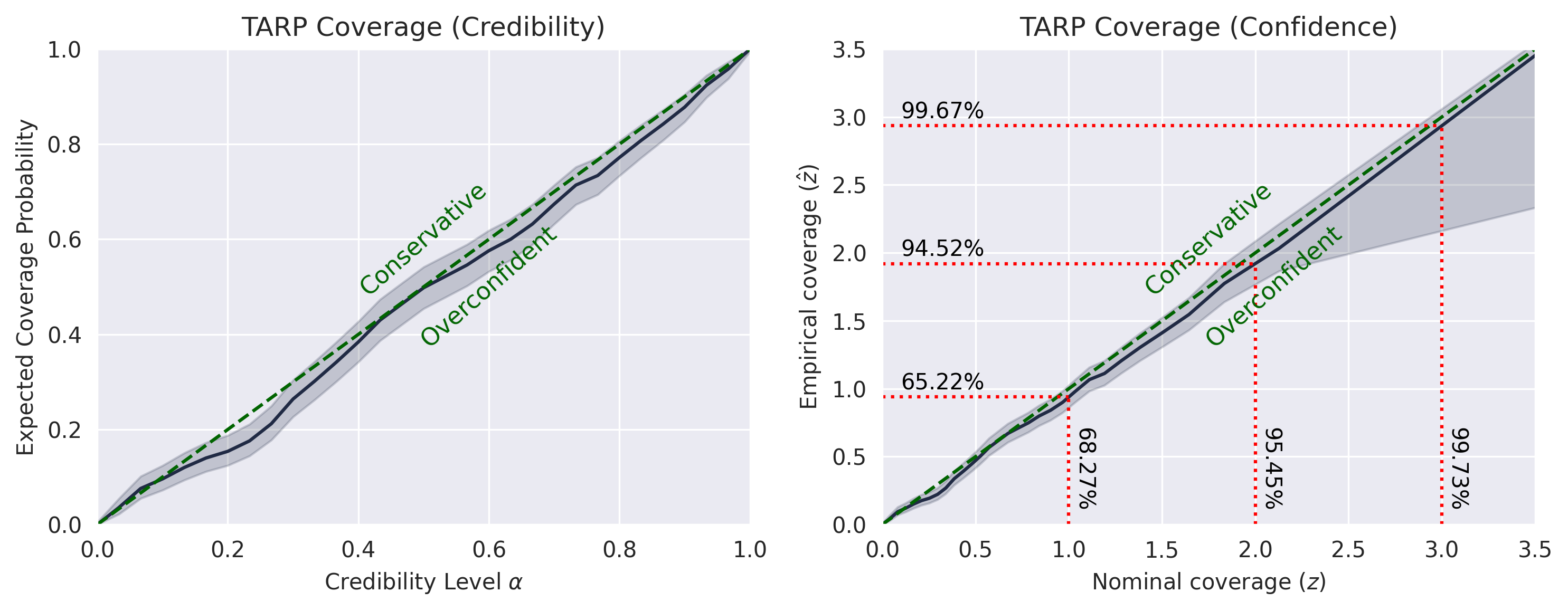
6.2. TARP (Test of Accuracy and Reliability of Posterior)

We calculate the Expected Coverage Probability (ECP) to assess the calibration of the posterior.

print("Running TARP diagnostic...")

# Calculate ECP and Alpha
tarp_result = run_tarp(
    thetas,
    posterior_samples,
    references=None,  # will be calculated automatically.
)

# Plot TARP
plot_tarp(tarp_result)
plt.title("TARP")
plt.show()

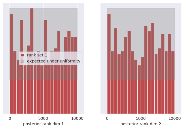
6.3. SBC (Simulation-Based Calibration)

We check the uniformity of the rank statistics.

print("Running SBC diagnostic...")

# Compute ranks
ranks, dap_samples = run_sbc(thetas, xs, posterior_samples)

# Plot SBC
f, ax = sbc_rank_plot(ranks, num_posterior_samples, plot_type="hist", num_bins=20)
plt.suptitle("SBC")
plt.show()

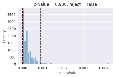
6.4. L-C2ST (Local Classifier 2-Sample Test)

We train a classifier to distinguish between true and sampled parameters.

print("Running L-C2ST diagnostic...")

# 1. Prepare data for LC2ST
# We use a slightly larger set for training the classifier, but single sample per observation
num_lc2st_data = 10000
data_lc2st = task.dataset["test"].with_format("jax")[:num_lc2st_data]
xs_lc2st = jnp.asarray(data_lc2st["xs"], dtype=jnp.bfloat16)
thetas_lc2st = jnp.asarray(data_lc2st["thetas"], dtype=jnp.bfloat16)

# Sample 1 posterior sample per observation
posterior_samples_lc2st = pipeline.sample(
    jax.random.PRNGKey(43), xs_lc2st, num_lc2st_data, use_ema=True
)

# Reshape
thetas_lc2st_flat = thetas_lc2st.reshape(thetas_lc2st.shape[0], -1)
xs_lc2st_flat = xs_lc2st.reshape(xs_lc2st.shape[0], -1)
posterior_samples_lc2st_flat = posterior_samples_lc2st.reshape(posterior_samples_lc2st.shape[0], -1)

# 2. Train the L-C2ST classifier
# Validation split happens inside LC2ST or we can hold out manually. 
# Here we hold out the last sample for visualization.
lc2st = LC2ST(
    thetas=thetas_lc2st_flat[:-1],
    xs=xs_lc2st_flat[:-1],
    posterior_samples=posterior_samples_lc2st_flat[:-1],
    classifier="mlp",
    num_ensemble=1,
)

print("Training classifier under null hypothesis...")
_ = lc2st.train_under_null_hypothesis()
print("Training classifier on observed data...")
_ = lc2st.train_on_observed_data()

# 3. Visualize on a held-out observation
x_o_star = xs_lc2st[-1:]
theta_o_star = thetas_lc2st[-1:]

# Sample many points for this specific observation to visualize the local score landscape
print("Sampling for visualization...")
post_samples_star = pipeline.sample(
    jax.random.PRNGKey(44), x_o_star[0], 10_000, use_ema=True
)

# Flatten for plotting
x_o_star_flat = x_o_star.reshape(1, -1)
post_samples_star_flat = np.array(
    post_samples_star.reshape(post_samples_star.shape[0], -1)
)

fig, ax = plot_lc2st(
    lc2st,
    post_samples_star_flat,
    x_o_star_flat,
)
plt.show()