EDM Diffusion Models#
Based on the article Elucidating the Design Space of Diffusion-Based Generative Models (Karras et al., 2022).
The EDM (Elucidated Diffusion Model) framework streamlines diffusion-based generative modeling by systematically disentangling the design choices — noise schedules, network parameterisation, loss weighting, and sampler construction — into a single, coherent recipe. While the score matching approach described previously uses the full stochastic reverse-time SDE for sampling, EDM instead emphasises the deterministic probability flow ODE as its primary sampling backbone.
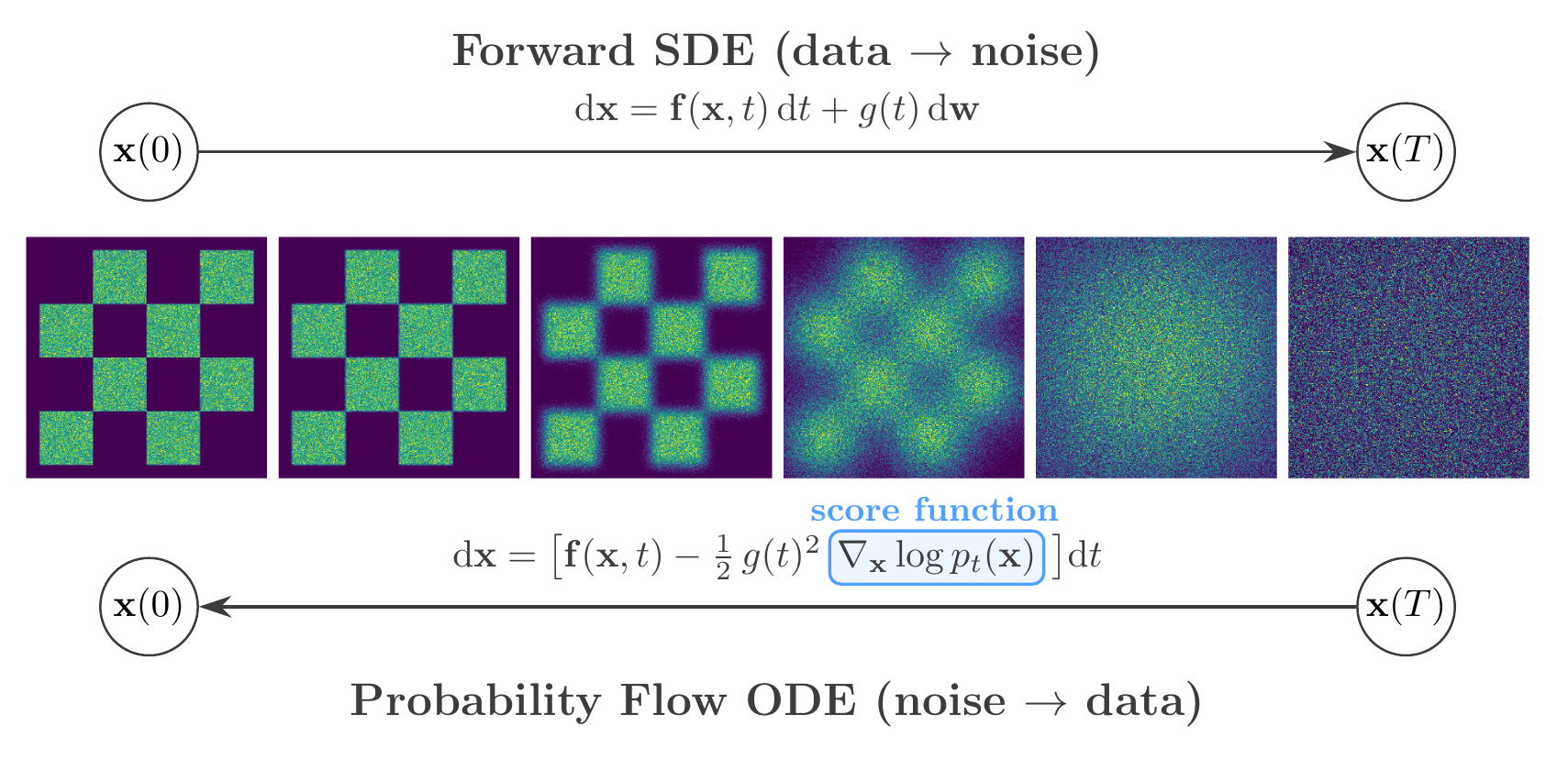
EDM framework. Top: the forward SDE progressively corrupts data into noise. Bottom: the probability flow ODE recovers data from noise deterministically, guided by the learned score function \(\nabla_{\mathbf{x}} \log p_t(\mathbf{x})\).#
From SDE to Probability Flow ODE#
Song et al. (2021) demonstrated that for every diffusion governed by an SDE of the form \(\mathrm{d}\mathbf{x} = \mathbf{f}(\mathbf{x},t)\,\mathrm{d}t + g(t)\,\mathrm{d}\mathbf{w}\), there exists a deterministic ODE — the probability flow ODE — whose trajectories share the same marginal distributions \(p_t(\mathbf{x})\) at every time \(t\):
This result follows from the Fokker–Planck equation associated with the SDE. Since the score function is the same one estimated via denoising score matching, a single trained network supports both SDE-based and ODE-based sampling.
Practical advantages of the ODE formulation:
Reproducibility: given a fixed initial noise vector, the trajectory to the generated sample is fully determined
Efficiency: adaptive-step ODE solvers (e.g. Runge–Kutta 45) can reduce the number of required network evaluations
Likelihood computation: the continuous change-of-variables formula yields exact log-likelihoods:
The EDM Design Space#
Karras et al. reformulated the probability flow ODE through a generalised parameterisation using a noise schedule \(\sigma(t)\) and a scale schedule \(s(t)\):
Different choices of \(s(t)\) and \(\sigma(t)\) recover all previously proposed noise schedules as special cases. In particular, the VP and VE SDEs from score matching correspond to specific schedule choices within this unified framework — they are not distinct models.
Network Preconditioning#
The central practical contribution of EDM is a principled preconditioning scheme. Rather than training \(F_\theta\) to predict the noise or the score directly — both of which suffer from scale-dependent error amplification — EDM wraps the raw network in \(\sigma\)-dependent scaling functions:
Each modulating function is derived from the requirement that both the effective input and target of \(F_\theta\) have unit variance across all noise levels:
Coefficient |
Formula |
Purpose |
|---|---|---|
\(c_\mathrm{in}(\sigma)\) |
\(1/\sqrt{\sigma^2 + \sigma_\mathrm{data}^2}\) |
Normalises the noisy input |
\(c_\mathrm{out}(\sigma)\) |
\(\sigma\,\sigma_\mathrm{data}/\sqrt{\sigma^2 + \sigma_\mathrm{data}^2}\) |
Normalises the effective training target |
\(c_\mathrm{skip}(\sigma)\) |
\(\sigma_\mathrm{data}^2/(\sigma^2 + \sigma_\mathrm{data}^2)\) |
Minimises error amplification |
\(c_\mathrm{noise}(\sigma)\) |
\(\tfrac{1}{4}\ln\sigma\) |
Empirical noise conditioning input |
These scalings ensure the network operates in a well-conditioned regime regardless of the noise level, leading to more stable training.
The relationship between the denoiser and the score is:
so learning to denoise at every intensity level \(\sigma\) implicitly learns the score function — the gradient of the log-probability density. This gradient points towards regions of higher data density, guiding the transformation from noise to data.
Training Loss#
The model is trained using a weighted denoising MSE objective over noise levels sampled from a log-normal distribution:
where \(\mathbf{y}\) is a clean sample, \(\mathbf{n} \sim \mathcal{N}(0, \sigma^2 I)\), and \(\lambda(\sigma) = (\sigma^2 + \sigma_\mathrm{data}^2)/(\sigma\,\sigma_\mathrm{data})^2\) equalises the effective contribution of each noise level.
Stochastic Sampling#
For sampling, EDM combines a 2nd-order Heun ODE integrator with optional stochastic noise injection. At each step, the solver:
Evaluates the denoiser \(D_\theta\) at the current noise level
Computes an Euler estimate
Applies a corrector step at the target noise level for improved accuracy (\(O(h^3)\) local truncation error)
Beyond purely deterministic sampling, EDM introduces a stochastic variant controlled by a set of hyperparameters:
\(S_\mathrm{churn}\): overall amount of noise reinjection per step
\(S_\mathrm{min}\), \(S_\mathrm{max}\): noise-level range for stochasticity
\(S_\mathrm{noise}\): modulates the standard deviation of injected noise
This controlled reinjection of stochasticity during sampling can correct errors accumulated during earlier steps, particularly at intermediate noise levels, and in practice often improves sample quality beyond what the purely deterministic solver achieves.
EDM trajectories on an unconditional 2D example. The probability flow ODE produces deterministic trajectories from noise (right) to data (left).#
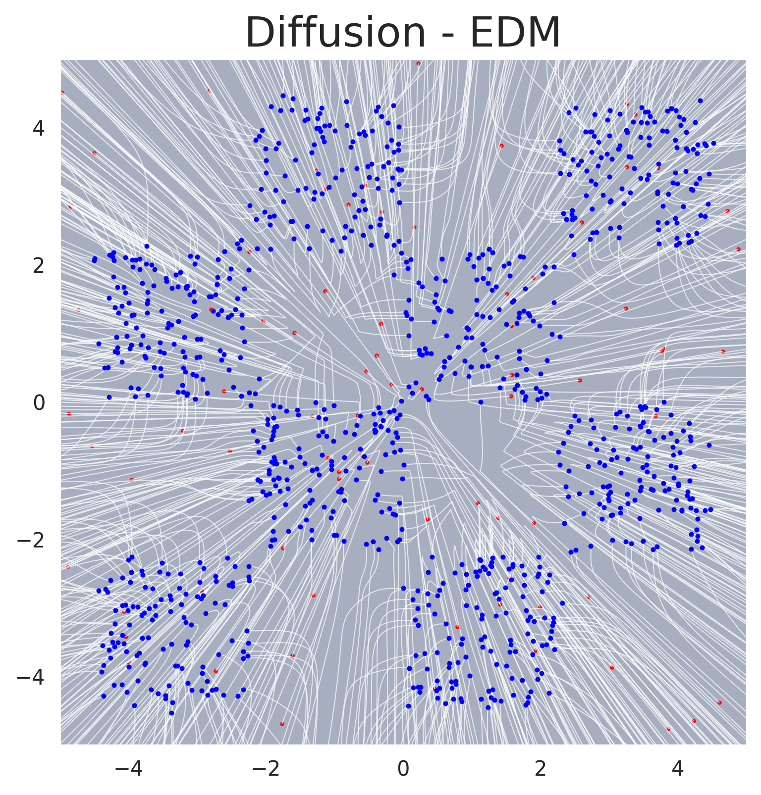
Sampling trajectories for EDM. Individual sample paths traced by the probability flow ODE, showing the deterministic denoising process.#
Application to SBI#
In the context of Simulation-Based Inference, the denoiser is trained conditionally as \(D_\psi(\boldsymbol{\theta}; \sigma, \mathbf{x})\), where \(\mathbf{x}\) is the observed data. The stochastic churn in the sampler is beneficial for SBI tasks involving complex posteriors: the explicit Langevin-like noise addition actively corrects approximation errors, preventing the trajectory from drifting off the target manifold. See the Conditional Density Estimation page for the full conditional formulation.
GenSBI Implementation#
The EDM framework is implemented in GenSBI’s DiffusionEDMMethod, which supports:
Standard EDM schedule as well as VP and VE schedules as special cases
EDMSolver: 2nd-order Heun sampler with configurable churn parameters (\(S_\mathrm{churn}\), \(S_\mathrm{min}\), \(S_\mathrm{max}\), \(S_\mathrm{noise}\))The solver can be swapped post-training without retraining the underlying model