Methods and Samplers in GenSBI#
GenSBI supports three generative methods for simulation-based inference:
Flow Matching — learns a velocity field and integrates an ODE from noise to data.
EDM Diffusion — learns a denoiser in σ-space (Karras et al., 2022).
Score Matching — learns the score function ∇ log p_t(x) (Song et al., 2021).
Each method has a default solver and one or more alternatives that can be swapped at sample time without retraining. This example trains one model per method and demonstrates all available sampling strategies.
We use the unified ConditionalPipeline API throughout, which is model-agnostic
and parameterized by a GenerativeMethod object.
# automatically install dependencies if using Colab
try: #check if we are using colab, if so install all the required software
    import google.colab
    colab=True
except:
    colab=False

if colab: # you may have to restart the runtime after installing the packages
    !uv pip install --quiet "gensbi[cuda12,examples]"
    !git clone --depth 1 https://github.com/aurelio-amerio/GenSBI-examples
    %cd GenSBI-examples/examples/methods_and_samplers
import os

# Set JAX backend (use 'cuda' for GPU, 'cpu' otherwise)
os.environ["JAX_PLATFORMS"] = "cuda"

import grain
import numpy as np
import jax
from jax import numpy as jnp
from numpyro import distributions as dist
from flax import nnx

# Unified pipeline and generative methods
from gensbi.recipes import ConditionalPipeline
from gensbi.core import FlowMatchingMethod, DiffusionEDMMethod, ScoreMatchingMethod

# Model
from gensbi.models import Flux1, Flux1Params

# Plotting
from gensbi.utils.plotting import plot_marginals
import matplotlib.pyplot as plt
Model parameters#
params = Flux1Params(
    in_channels=1,
    vec_in_dim=None,
    context_in_dim=1,
    mlp_ratio=3,
    num_heads=4,
    depth=4,
    depth_single_blocks=8,
    val_emb_dim=10,
    id_emb_dim=4,
    qkv_bias=True,
    dim_obs=dim_obs,
    dim_cond=dim_cond,
    id_embedding_strategy=("absolute", "absolute"),
    id_merge_mode="concat",
    rngs=nnx.Rngs(default=42),
    param_dtype=jnp.float32,
)
Section 1: Flow Matching#
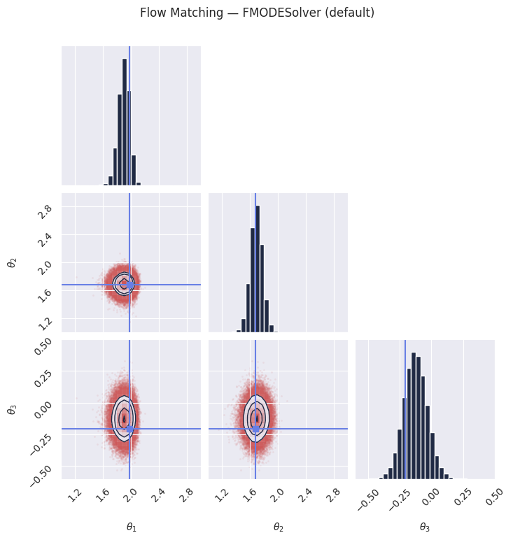
Flow Matching learns a velocity field \(v_\theta(t, x)\) that transports samples from a simple prior (Gaussian noise at \(t=0\)) to the data distribution (at \(t=1\)) via an ordinary differential equation (ODE).
Default solver:
FMODESolver— deterministic ODE integration (Euler or Dopri5).Alternative solvers (SDE-based, stochastic):
ZeroEndsSolver— diffusion vanishes at both time endpoints (arXiv:2410.02217).NonSingularSolver— non-singular diffusion coefficient (arXiv:2410.02217).
The SDE solvers can sometimes improve sample diversity at the cost of
additional stochasticity. The prior statistics (mu0, sigma0) are auto-provided;
only the diffusion strength parameter alpha must be specified.
model_fm = Flux1(params)

method_fm = FlowMatchingMethod()

training_config_fm = ConditionalPipeline.get_default_training_config()
training_config_fm["nsteps"] = 10000
training_config_fm["checkpoint_dir"] = os.path.join(os.getcwd(), "checkpoints", "flow")

pipeline_fm = ConditionalPipeline(
    model_fm,
    train_dataset_grain,
    val_dataset_grain,
    dim_obs=dim_obs,
    dim_cond=dim_cond,
    method=method_fm,
    training_config=training_config_fm,
)
# Uncomment the following lines to train the model.
# Once trained, the model is saved to checkpoints/flow and can be restored below.
rngs = nnx.Rngs(42)
# pipeline_fm.train(rngs, save_model=True)
pipeline_fm.restore_model()
# The default solver for flow matching is the FMODESolver, which performs deterministic
# ODE integration from noise (t=0) to data (t=1).
samples_fm = pipeline_fm.sample(rngs.sample(), x_o, nsamples=100_000)
samples_fm = unnormalize(samples_fm, means[:dim_obs], stds[:dim_obs])
plot_marginals(
    np.array(samples_fm[..., 0]),
    gridsize=30,
    true_param=np.array(true_theta[0, :, 0]),
    range=plot_range,
)
plt.suptitle("Flow Matching — FMODESolver (default)", y=1.02)
plt.savefig("fm_ode_marginals.png", dpi=100, bbox_inches="tight")
plt.show()
# The ZeroEndsSolver adds stochastic noise during sampling. The diffusion coefficient
# vanishes at both t=0 and t=1, ensuring clean endpoints.
# Required kwarg: alpha (diffusion strength). mu0/sigma0 are auto-provided by the prior.
from gensbi.flow_matching.solver import ZeroEndsSolver

solver_kwargs_ze = {
    "alpha": 0.2,  # diffusion strength
}

samples_fm_ze = pipeline_fm.sample(
    rngs.sample(),
    x_o,
    nsamples=100_000,
    solver=(ZeroEndsSolver, solver_kwargs_ze),
)
samples_fm_ze = unnormalize(samples_fm_ze, means[:dim_obs], stds[:dim_obs])
plot_marginals(
    np.array(samples_fm_ze[..., 0]),
    gridsize=30,
    true_param=np.array(true_theta[0, :, 0]),
    range=plot_range,
)
plt.suptitle("Flow Matching — ZeroEndsSolver (SDE)", y=1.02)
plt.savefig("fm_zeroends_marginals.png", dpi=100, bbox_inches="tight")
plt.show()

# The NonSingularSolver uses a non-singular diffusion coefficient, which can provide
# different sample quality characteristics compared to ZeroEndsSolver.
# It takes the same kwargs as ZeroEndsSolver.
from gensbi.flow_matching.solver import NonSingularSolver

solver_kwargs_ns = {
    "alpha": 0.2,
}

samples_fm_ns = pipeline_fm.sample(
    rngs.sample(),
    x_o,
    nsamples=100_000,
    solver=(NonSingularSolver, solver_kwargs_ns),
)
samples_fm_ns = unnormalize(samples_fm_ns, means[:dim_obs], stds[:dim_obs])
plot_marginals(
    np.array(samples_fm_ns[..., 0]),
    gridsize=30,
    true_param=np.array(true_theta[0, :, 0]),
    range=plot_range,
)
plt.suptitle("Flow Matching — NonSingularSolver (SDE)", y=1.02)
plt.savefig("fm_nonsingular_marginals.png", dpi=100, bbox_inches="tight")
plt.show()

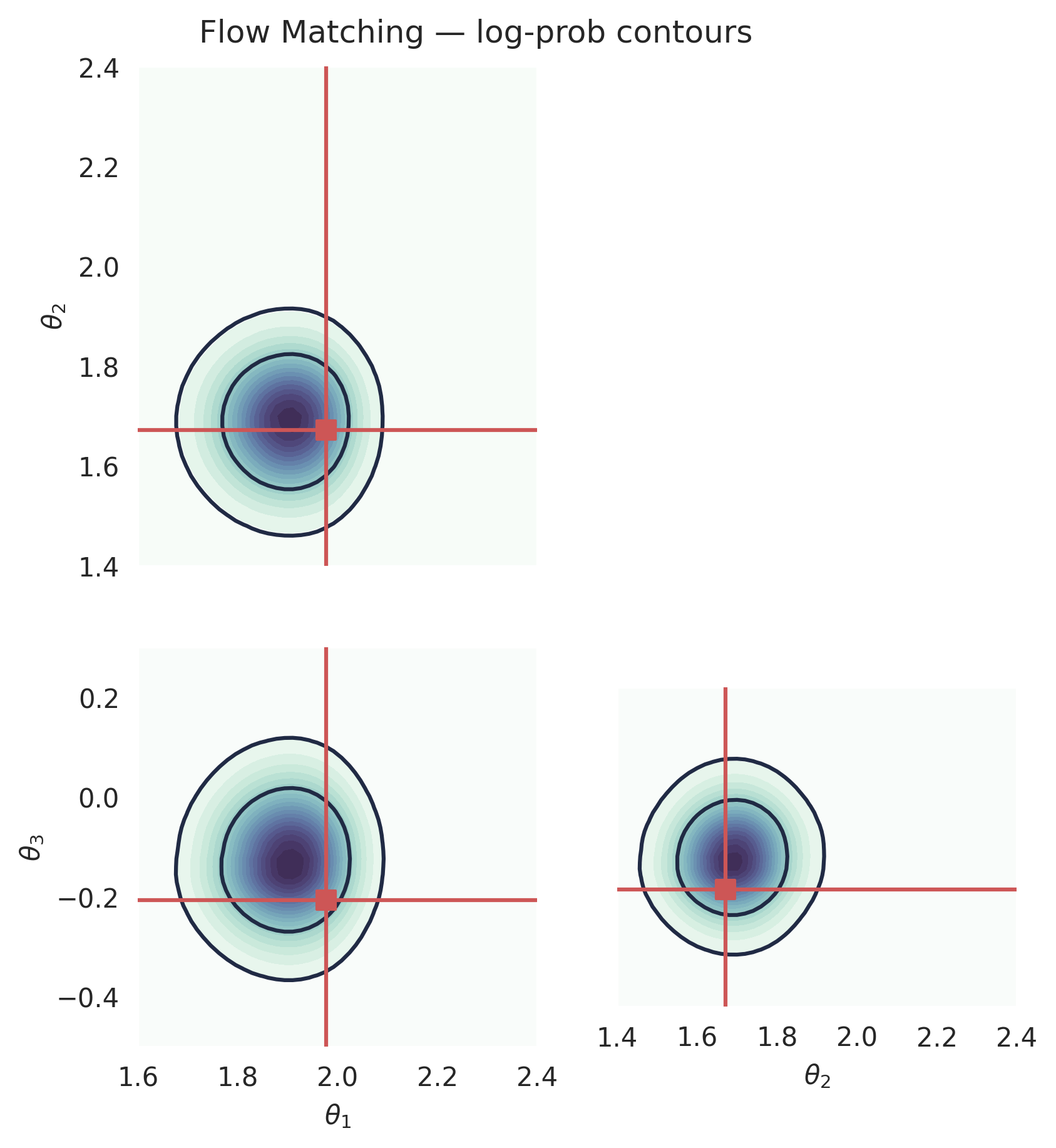
Computing the log-prob (Flow Matching)#
Flow matching supports exact log-probability evaluation via the continuous change-of-variables formula. This requires solving an ODE backward, so it is more expensive than sampling, but it gives the exact (approximate) posterior density at any point.
from gensbi.utils.plotting import _plot_2d_dist_contour
# Build a meshgrid in *unnormalized* space, then normalize for the pipeline.
# The plot_range we used for marginals is a good guide for the grid extent.
theta1_raw = np.linspace(1.6, 2.4, 50)
theta2_raw = np.linspace(1.4, 2.4, 51)
theta3_raw = np.linspace(-0.5, 0.3, 52)

# Normalize to the training data statistics (obs dims only)
means_obs = means[:dim_obs, :]
stds_obs = stds[:dim_obs, :]

theta1 = (theta1_raw - means_obs[0, 0].item()) / stds_obs[0, 0].item()
theta2 = (theta2_raw - means_obs[1, 0].item()) / stds_obs[1, 0].item()
theta3 = (theta3_raw - means_obs[2, 0].item()) / stds_obs[2, 0].item()

tt1, tt2, tt3 = jnp.meshgrid(theta1, theta2, theta3, indexing="ij")

x_1 = jnp.stack([tt1.ravel(), tt2.ravel(), tt3.ravel()], axis=-1)[..., None]
logp_fm = pipeline_fm.log_prob(x_1, x_o, use_ema=True)
prob_fm = jnp.exp(logp_fm).reshape((len(theta1_raw), len(theta2_raw), len(theta3_raw)))

# since we did a change of variables, p(x_norm) = p(x)*|det(J)|, where J is the jacobian of the change of variables
# we are interested in plotting p(x)
# J = stds_obs, so we need to divide by the product of stds
prob_fm = prob_fm / jnp.prod(stds_obs.flatten())

# Integrate out one dimension to get 2D marginal distributions
prob12_fm = jnp.trapezoid(prob_fm, x=theta3, axis=2)
prob13_fm = jnp.trapezoid(prob_fm, x=theta2, axis=1)
prob23_fm = jnp.trapezoid(prob_fm, x=theta1, axis=0)

fig, axes = plt.subplots(2, 2, figsize=(6, 6))

ax = axes[1, 0]
_plot_2d_dist_contour(theta1_raw, theta3_raw, prob13_fm.T, ax=ax,
                      true_param=[true_theta[:, 0], true_theta[:, 2]])
ax.set_xlabel(r"$\theta_1$")
ax.set_ylabel(r"$\theta_3$")


ax = axes[1, 1]
_plot_2d_dist_contour(theta2_raw, theta3_raw, prob23_fm.T, ax=ax,
                      true_param=[true_theta[:, 1], true_theta[:, 2]])
ax.set_xlabel(r"$\theta_2$")
ax.set_ylabel("")
ax.set_yticks([])


ax = axes[0, 0]
_plot_2d_dist_contour(theta1_raw, theta2_raw, prob12_fm.T, ax=ax,
                      true_param=[true_theta[:, 0], true_theta[:, 1]])
ax.set_xlabel("")
ax.set_xticks([])
ax.set_ylabel(r"$\theta_2$")


axes[0, 1].set_visible(False)

fig.subplots_adjust(hspace=0.05, wspace=0.2, left=0.2, right=0.98, top=0.98, bottom=0.06)
for ax in axes.ravel():
    ax.set_aspect("equal", adjustable="box")
    # ax.set_aspect("equal")

plt.suptitle("Flow Matching — log-prob contours", y=1.02)
plt.savefig("fm_log_prob.png", dpi=300, bbox_inches="tight")
plt.show()
del model_fm, pipeline_fm
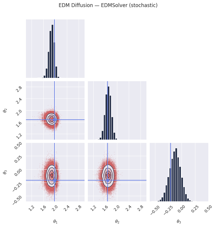
Section 2: EDM Diffusion#
EDM Diffusion (Karras et al., 2022) learns a denoiser \(D_\theta(x; \sigma)\) in \(\sigma\)-space. The training noise schedule can use one of three prescriptions:
DiffusionEDMMethod()— default EDM scheduler (recommended)DiffusionEDMMethod(sde="VP")— Variance Preserving schedulerDiffusionEDMMethod(sde="VE")— Variance Exploding scheduler
The model can be trained with any of these three prescriptions, and then sampled using any of the three as well. However, the EDM scheduler is recommended for both training and sampling. The scheduler variants are training-time choices that affect the noise schedule used during the diffusion process.
Solver: EDMSolver is the only available solver for EDM. It implements the
stochastic denoising sampler from Karras et al., 2022.
model_edm = Flux1(params)

# Default EDM scheduler (recommended for both training and sampling)
method_edm = DiffusionEDMMethod()
# Alternative training schedulers (uncomment to use):
# method_edm = DiffusionEDMMethod(sde="VP")  # Variance Preserving
# method_edm = DiffusionEDMMethod(sde="VE")  # Variance Exploding

training_config_edm = ConditionalPipeline.get_default_training_config()
training_config_edm["nsteps"] = 10000
training_config_edm["checkpoint_dir"] = os.path.join(os.getcwd(), "checkpoints", "edm")

pipeline_edm = ConditionalPipeline(
    model_edm,
    train_dataset_grain,
    val_dataset_grain,
    dim_obs=dim_obs,
    dim_cond=dim_cond,
    method=method_edm,
    training_config=training_config_edm,
)
# Uncomment the following lines to train the model.
# Once trained, the model is saved to checkpoints/edm and can be restored below.
rngs = nnx.Rngs(42)
# pipeline_edm.train(rngs, save_model=True)
pipeline_edm.restore_model()
# The EDMSolver implements the stochastic denoising sampler from Karras et al., 2022. Defaults to algorithm 1 (deterministic)
# It progressively denoises samples following a noise schedule from high to low sigma.
samples_edm = pipeline_edm.sample(rngs.sample(), x_o, nsamples=100_000)
samples_edm = unnormalize(samples_edm, means[:dim_obs], stds[:dim_obs])
plot_marginals(
    np.array(samples_edm[..., 0]),
    gridsize=30,
    true_param=np.array(true_theta[0, :, 0]),
    range=plot_range,
)
plt.suptitle("EDM Diffusion — EDMSolver (default - deterministic)", y=1.02)
plt.savefig("edm_marginals.png", dpi=100, bbox_inches="tight")
plt.show()

# Setting S_churn != 0 will adopt a predictor-corrector stochastic sampling procedure, according to algorithm 2 of the paper
samples_edm_stochastic = pipeline_edm.sample(rngs.sample(), x_o, nsamples=100_000, S_churn=30)
samples_edm_stochastic = unnormalize(samples_edm_stochastic, means[:dim_obs], stds[:dim_obs])
plot_marginals(
    np.array(samples_edm_stochastic[..., 0]),
    gridsize=30,
    true_param=np.array(true_theta[0, :, 0]),
    range=plot_range,
)
plt.suptitle("EDM Diffusion — EDMSolver (stochastic)", y=1.02)
plt.savefig("edm_marginals_stochastic.png", dpi=100, bbox_inches="tight")
plt.show()
Note: EDM diffusion does not currently support exact log-probability evaluation. Only flow matching and score matching provide this functionality via their ODE formulations.
del model_edm, pipeline_edm
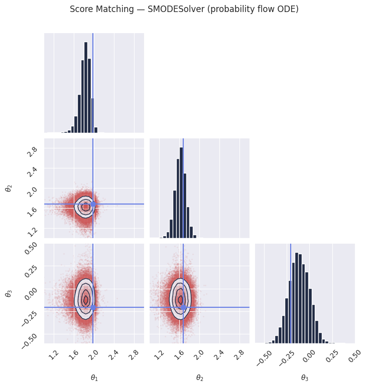
Section 3: Score Matching#
Score Matching (Song et al., 2021) learns the score function \(\nabla \log p_t(x)\), which points toward regions of higher data density. Samples are generated by running a reverse-time SDE from noise back to data.
The SDE formulation can be either:
ScoreMatchingMethod()— Variance Preserving (VP) SDE (default)ScoreMatchingMethod(sde_type="VE")— Variance Exploding (VE) SDE
Solvers:
SMSDESolver(default) — reverse-time SDE, generates stochastic samples.SMODESolver— probability flow ODE, generates deterministic samples from the same learned score function. Useful when reproducibility or lower variance is desired.
model_sm = Flux1(params)

# Default: Variance Preserving (VP) SDE
method_sm = ScoreMatchingMethod()
# Alternative: Variance Exploding (VE) SDE (uncomment to use)
# method_sm = ScoreMatchingMethod(sde_type="VE")

training_config_sm = ConditionalPipeline.get_default_training_config()
training_config_sm["nsteps"] = 50000
training_config_sm["checkpoint_dir"] = os.path.join(os.getcwd(), "checkpoints", "sm")

pipeline_sm = ConditionalPipeline(
    model_sm,
    train_dataset_grain,
    val_dataset_grain,
    dim_obs=dim_obs,
    dim_cond=dim_cond,
    method=method_sm,
    training_config=training_config_sm,
)
# Uncomment the following lines to train the model.
# Once trained, the model is saved to checkpoints/sm and can be restored below.
rngs = nnx.Rngs(42)
# pipeline_sm.train(rngs, save_model=True)
pipeline_sm.restore_model()
# The default solver for score matching generates stochastic samples by running the
# reverse-time SDE. Each call with a different key produces a different set of samples.
samples_sm = pipeline_sm.sample(rngs.sample(), x_o, nsamples=100_000)
samples_sm = unnormalize(samples_sm, means[:dim_obs], stds[:dim_obs])
plot_marginals(
    np.array(samples_sm[..., 0]),
    gridsize=30,
    true_param=np.array(true_theta[0, :, 0]),
    range=plot_range,
)
plt.suptitle("Score Matching — SMSDESolver (default, reverse SDE)", y=1.02)
plt.savefig("sm_sde_marginals.png", dpi=100, bbox_inches="tight")
plt.show()

# The probability flow ODE produces deterministic samples from the same learned score
# function. This can be useful when you want reproducible results or lower variance.
from gensbi.diffusion.solver import SMODESolver

samples_sm_pf = pipeline_sm.sample(
    rngs.sample(),
    x_o,
    nsamples=100_000,
    solver=(SMODESolver, {}),
)
samples_sm_pf = unnormalize(samples_sm_pf, means[:dim_obs], stds[:dim_obs])
plot_marginals(
    np.array(samples_sm_pf[..., 0]),
    gridsize=30,
    true_param=np.array(true_theta[0, :, 0]),
    range=plot_range,
)
plt.suptitle("Score Matching — SMODESolver (probability flow ODE)", y=1.02)
plt.savefig("sm_pf_marginals.png", dpi=100, bbox_inches="tight")
plt.show()
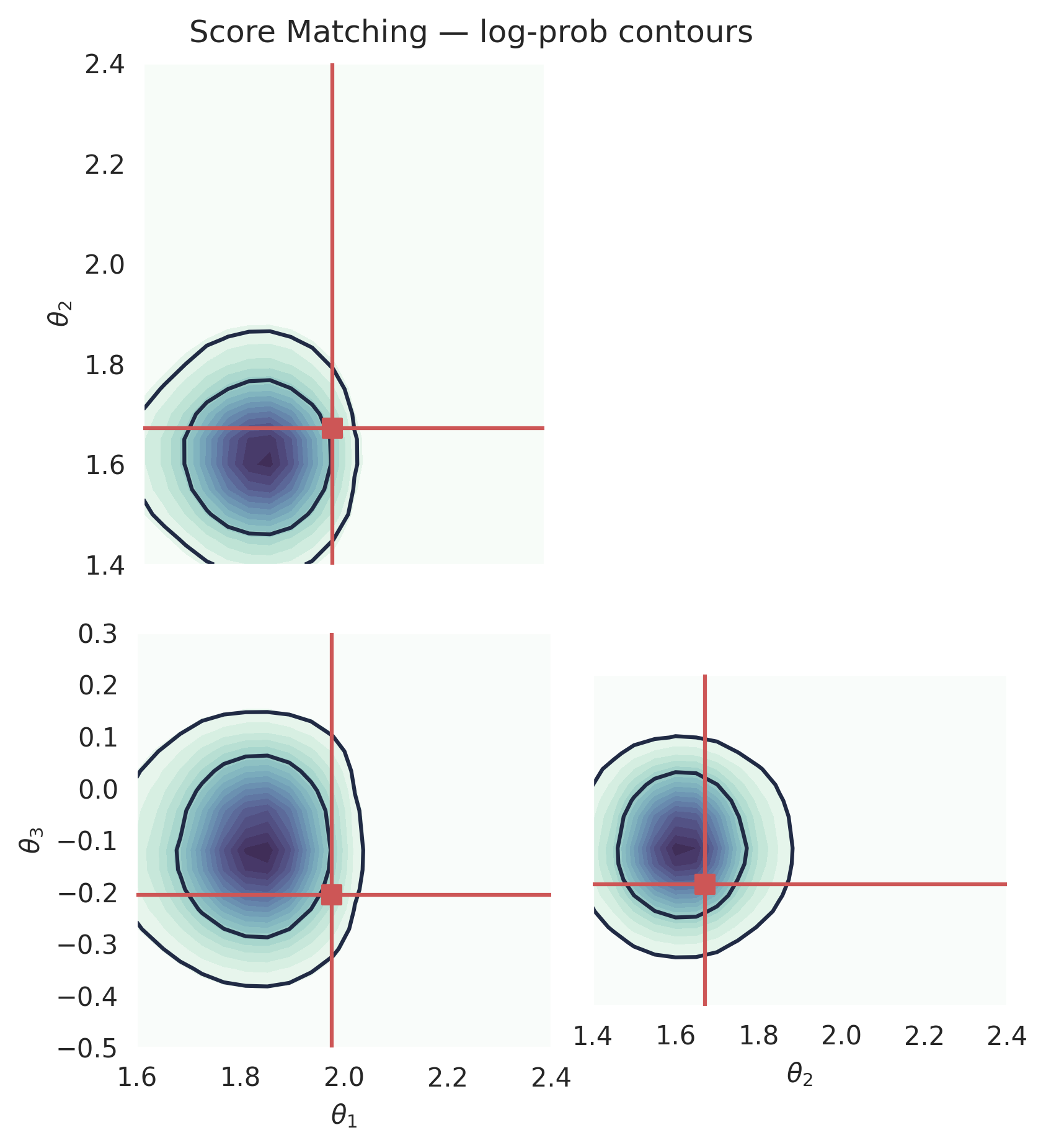
Computing the log-prob (Score Matching)#
Score matching also supports exact log-probability evaluation via the
probability flow ODE formulation. Internally, pipeline.log_prob() uses
SMODESolver regardless of the default sampling solver.
# We reuse the same unnormalized grid ranges defined in the FM section.
from gensbi.utils.plotting import _plot_2d_dist_contour

theta1_raw = np.linspace(1.6, 2.4, 20)
theta2_raw = np.linspace(1.4, 2.4, 21)
theta3_raw = np.linspace(-0.5, 0.3, 22)

means_obs = means[:dim_obs, :]
stds_obs = stds[:dim_obs, :]

theta1 = (theta1_raw - means_obs[0, 0].item()) / stds_obs[0, 0].item()
theta2 = (theta2_raw - means_obs[1, 0].item()) / stds_obs[1, 0].item()
theta3 = (theta3_raw - means_obs[2, 0].item()) / stds_obs[2, 0].item()

tt1, tt2, tt3 = jnp.meshgrid(theta1, theta2, theta3, indexing="ij")
x_1 = jnp.stack([tt1.ravel(), tt2.ravel(), tt3.ravel()], axis=-1)[..., None]
logp_sm = pipeline_sm.log_prob(x_1, x_o, use_ema=True, method="Euler")
prob_sm = jnp.exp(logp_sm).reshape((len(theta1_raw), len(theta2_raw), len(theta3_raw)))
prob_sm = prob_sm / jnp.prod(stds_obs.flatten())

prob12_sm = jnp.trapezoid(prob_sm, x=theta3, axis=2)
prob13_sm = jnp.trapezoid(prob_sm, x=theta2, axis=1)
prob23_sm = jnp.trapezoid(prob_sm, x=theta1, axis=0)

fig, axes = plt.subplots(2, 2, figsize=(6, 6))

ax = axes[1, 0]
_plot_2d_dist_contour(theta1_raw, theta3_raw, prob13_sm.T, ax=ax,
                      true_param=[true_theta[:, 0], true_theta[:, 2]])
ax.set_xlabel(r"$\theta_1$")
ax.set_ylabel(r"$\theta_3$")

ax = axes[1, 1]
_plot_2d_dist_contour(theta2_raw, theta3_raw, prob23_sm.T, ax=ax,
                      true_param=[true_theta[:, 1], true_theta[:, 2]])
ax.set_xlabel(r"$\theta_2$")
ax.set_ylabel("")
ax.set_yticks([])

ax = axes[0, 0]
_plot_2d_dist_contour(theta1_raw, theta2_raw, prob12_sm.T, ax=ax,
                      true_param=[true_theta[:, 0], true_theta[:, 1]])
ax.set_xlabel("")
ax.set_xticks([])
ax.set_ylabel(r"$\theta_2$")

axes[0, 1].set_visible(False)

fig.subplots_adjust(hspace=0.05, wspace=0.1, left=0.2, right=0.98, top=0.98, bottom=0.06)
for ax in axes.ravel():
    ax.set_aspect("equal", adjustable="box")

plt.suptitle("Score Matching — log-prob contours", y=1.02)
plt.savefig("sm_log_prob.png", dpi=300, bbox_inches="tight")
plt.show()
del model_sm, pipeline_sm