Two Moons MAF NLE Example#

Notice: If you find any errors, please open an issue on the GenSBI-examples GitHub repository.

This notebook demonstrates Neural Likelihood Estimation (NLE) on the Two Moons task using a MAF (Masked Autoregressive Flow) in JAX and Flax.

NLE in one paragraph. Instead of learning the posterior \(p(\theta \mid x)\) directly (as in NPE), NLE learns the likelihood \(q(x \mid \theta)\) with a conditional density estimator. At inference time the posterior is recovered by combining the learned likelihood with the prior, \(p(\theta \mid x_o) \propto q(x_o \mid \theta)\, p(\theta)\), and drawing samples from this (unnormalized) density with a sampler. This decouples learning the density from sampling the posterior, and lets a single trained likelihood serve any observation.

Why Two Moons + MAF + a multimodal sampler. Two Moons has a 2-D parameter \(\theta\) and a 2-D observation \(x\). Its posterior is famously multimodal: for a single observation it collapses onto two disjoint crescent (“moon”) shapes. A compact MAF captures the likelihood well, but a single MCMC chain started in one crescent would never cross to the other, so we need a sampler that populates all modes. This notebook showcases two such samplers side by side:

Tempered SMC (labelled MCMC in the figures) — a particle cloud walked from the prior to the posterior along \(p(\theta)\, q(x_o \mid \theta)^\beta\) for \(\beta: 0 \to 1\), populating every mode.
Nested Sampling (labelled NS) — blackjax nested slice sampling, which walks live points from the prior inward, handles the multimodal posterior without tempering, and additionally returns a log-evidence estimate.

Both recover the same two-crescent posterior, and their log-evidence estimates serve as a mutual cross-check.

NLE convention (mirror of NPE): obs = x, cond = theta, so the flow models \(q(x \mid \theta)\). This is the only substantive difference from an NPE example; the flow and pipeline are otherwise identical.

Table of Contents#

Section	Description
1. Introduction & Setup	Overview, environment, device
2. Task & Data Preparation	Define task, swap obs/cond for NLE, build datasets
3. Model Configuration & Definition	Load config, build the MAF with its params class, standardize
4. Training	Train (commented out) or restore the checkpoint
5. Posterior Sampling with Tempered SMC (MCMC)	Prior + learned likelihood, tempered SMC, visualize posterior
6. Posterior Sampling with Nested Sampling (NS)	Same posterior via nested sampling, log-evidence cross-check

1. Introduction & Setup#

In this section, we set up the computational environment, import the required libraries, and configure JAX for CPU or GPU usage. Compatibility with Google Colab is also ensured.

# Check if running on Colab and install dependencies if needed
try:
    import google.colab
    colab = True
except ImportError:
    colab = False

if colab:
    # Install required packages and clone the repository
    !uv pip install --quiet "gensbi[cuda12,examples]" "sbibm-jax[loader]"
    !git clone --depth 1 https://github.com/aurelio-amerio/GenSBI-examples
    %cd GenSBI-examples/examples/sbi-benchmarks/two_moons/maf_NLE

import os
# select device

os.environ["JAX_PLATFORMS"] = "cuda"
# os.environ["JAX_PLATFORMS"] = "cpu" 

import yaml
import numpy as np
import matplotlib.pyplot as plt

import jax
import jax.numpy as jnp
from flax import nnx

from gensbi.normalizing_flows import Affine, RQSpline
from gensbi.models import MAFlow, MAFlowParams
from gensbi.recipes import ConditionalFlowPipeline
from gensbi.inference import NLEPosterior, TemperedSMC, NestedSampler
from gensbi.utils.plotting import plot_marginals
from sbibm_jax.data import TaskDataset
from sbibm_jax.tasks import get_task

2. Task & Data Preparation#

In this section, we define the Two Moons task, visualize the reference posterior, and build the training/validation datasets. The key NLE-specific step is swapping obs and cond so the flow learns \(q(x \mid \theta)\).

# By default we restore the released checkpoint instead of training from scratch.
restore_model = True
train_model = False

# Resolve paths relative to this notebook. The checkpoint and config ship in the repo.
notebook_path = os.getcwd()
checkpoint_dir = os.path.join(notebook_path, "checkpoints")
config_path = os.path.join(notebook_path, "config", "config_maf_nle.yaml")

with open(config_path) as f:
    config = yaml.safe_load(f)

task_name = config["task_name"]   # "two_moons"

# Conditional task. We keep the raw loader (normalize=False): x is standardized
# *inside* the flow (see Section 3), not by the data loader.
task = TaskDataset(task_name, kind="conditional", normalize=False, use_prefetching=False)

# NLE: the autoregressive target is the observation x, conditioned on theta.
dim_obs, dim_cond = task.dim_x, task.dim_theta
print(f"dim_obs (x) = {dim_obs}, dim_cond (theta) = {dim_cond}")

# reference posterior samples (theta) for one observation
obs, reference_samples = task.get_reference(num_observation=8)

# plot the reference posterior over the 2-D theta (the two-moons crescents)
plot_marginals(np.asarray(reference_samples, dtype=np.float32), gridsize=50, plot_levels=False, backend="seaborn")
plt.show()

def swap_obs_cond(batch):
    """Map a conditional batch (theta, x) -> (x, theta) for NLE.

    TaskDataset's conditional collate yields (theta, x); the pipeline reads
    `obs, cond = batch`. NLE models q(x | theta), so obs must be x and cond theta.
    """
    theta, x = batch
    return x, theta

# Build the datasets and apply the NLE obs/cond swap. nsamples must be < task.max_samples.
train_cfg = config["training"]
batch_size = int(train_cfg["batch_size"])
nsamples = int(train_cfg["nsamples"])

train_ds = task.get_train_loader(batch_size, num_samples=nsamples).map(swap_obs_cond)
val_ds = task.get_val_loader(512).map(swap_obs_cond)

3. Model Configuration & Definition#

In this section, we build the MAF from its parameter class MAFlowParams, wrap it in a ConditionalFlowPipeline, and set the in-flow standardization from the dataset statistics.

MAFlowParams is the single source of truth for the architecture. A MAF stacks n_layers autoregressive transforms, each parameterized by a small MLP (nn_width × nn_depth) and separated by a fixed permutation so every coordinate gets conditioned on the others across the stack. The elementwise transformer sets how each coordinate is warped: RQSpline (a monotonic rational-quadratic spline with num_bins knots) is far more expressive than a plain Affine shift-and-scale, which matters for the curved Two Moons likelihood. cond_dim is how theta enters each conditioner.

model_cfg = config["model"]

def build_transformer(model_cfg):
    """Return the elementwise transformer named in the model config."""
    name = str(model_cfg.get("transformer", "rqspline")).lower()
    if name == "affine":
        return Affine()
    if name == "rqspline":
        return RQSpline(num_bins=int(model_cfg.get("num_bins", 8)))
    raise ValueError(f"unknown transformer {name!r} (expected 'affine' or 'rqspline')")

def build_flow(rngs, dim_obs, dim_cond, model_cfg):
    """Instantiate the MAF from the model config via the MAFlowParams class.

    For NLE, dim == dim_obs (the autoregressive target x) and cond_dim == dim_cond (theta).
    """
    transformer = build_transformer(model_cfg)
    return MAFlow(MAFlowParams(
        rngs=rngs,
        dim=dim_obs,
        cond_dim=dim_cond,
        n_layers=int(model_cfg.get("n_layers", 8)),
        transformer=transformer,
        nn_width=int(model_cfg.get("nn_width", 64)),
        nn_depth=int(model_cfg.get("nn_depth", 2)),
        permutation=str(model_cfg.get("permutation", "reverse")),
        standardize=bool(model_cfg.get("standardize", True)),
        zero_init=bool(model_cfg.get("zero_init", True)),
    ))

flow = build_flow(nnx.Rngs(0), dim_obs, dim_cond, model_cfg)

# Training config: pipeline defaults overlaid with the YAML optimizer + training sections.
# The pipeline reads these eagerly, and uses `experiment_id` + `checkpoint_dir` to locate
# the checkpoint when restoring.
training_config = ConditionalFlowPipeline.get_default_training_config()
training_config.update(config.get("optimizer", {}))
training_config.update(config.get("training", {}))
training_config["checkpoint_dir"] = checkpoint_dir

pipeline = ConditionalFlowPipeline(
    flow, train_ds, val_ds, dim_obs, dim_cond, training_config=training_config
)

# In-flow standardization: x (the obs/target) is standardized inside the flow using the
# precomputed dataset statistics, so we don't fit them on the fly. The EMA copy averages
# only Params, so its non-Param Standardize buffer must be set explicitly too.
mean = jnp.asarray(task.x_mean).reshape(dim_obs)
std = jnp.asarray(task.x_std).reshape(dim_obs)

pipeline.model.set_standardization(mean, std)
pipeline.ema_model.set_standardization(mean, std)
pipeline._standardized = True  # suppress the train-time "did you fit?" warning

4. Training#

Training is shown but commented out by default; we restore the released checkpoint instead. Flip restore_model / train_model in Section 2 (or uncomment below) to train from scratch — on a GPU this takes a while for the configured nsteps.

# if train_model:
#     pipeline.train(nnx.Rngs(0))

if restore_model:
    pipeline.restore_model()

5. Posterior Sampling with Tempered SMC (MCMC)#

NLE recovers the posterior as learned likelihood × prior, then samples it. Two pieces matter:

The prior must validate its support. get_prior_dist() ships with validate_args=False, so its log_prob returns the in-support constant everywhere and would not bound the potential — the sampler would then wander outside the prior box and the posterior would be wrong. Re-enabling validation makes log_prob = -inf outside the support, confining the sampler to the box.
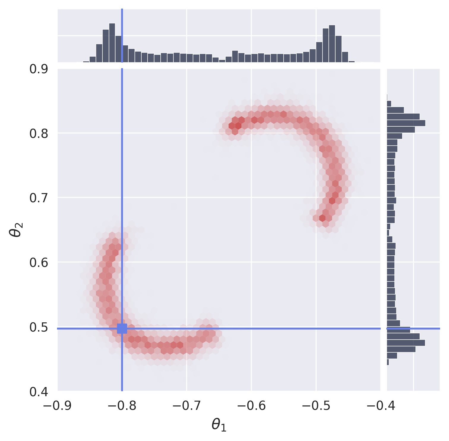
The sampler must be multimodal. TemperedSMC walks a particle cloud along \(p(\theta)\, q(x_o \mid \theta)^\beta\) for \(\beta: 0 \to 1\), populating both crescents. num_particles is the number of posterior samples returned. Passing return_info=True also gives us the SMC log-evidence estimate, which we compare against nested sampling in Section 6.

def build_prior(task_name, validate_args=True):
    """Task prior over theta with out-of-support log_prob = -inf (bounds the NLE potential)."""
    prior = get_task(task_name).get_prior_dist()
    prior._validate_args = validate_args
    if hasattr(prior, "base_dist"):          # Independent wraps a base distribution
        prior.base_dist._validate_args = validate_args
    return prior

prior = build_prior(task_name)

# NLEPosterior holds the (EMA) likelihood flow + prior; the sampler is supplied at sample time.
posterior = NLEPosterior(pipeline.ema_model, prior)

sampler_cfg = config["sampler"]
smc_sampler = TemperedSMC(
    num_particles=int(sampler_cfg.get("num_particles", 20000)),
    target_ess=float(sampler_cfg.get("target_ess", 0.9)),
    num_mcmc_steps=int(sampler_cfg.get("num_mcmc_steps", 10)),
    inner_kernel=str(sampler_cfg.get("inner_kernel", "mclmc")),  # mclmc | nuts
    inner_step_size=float(sampler_cfg.get("inner_step_size", 0.1)),
    inner_num_integration_steps=int(sampler_cfg.get("inner_num_integration_steps", 5)),
)

# Pick an observation, sample its posterior, and keep the true parameter for reference.
idx = int(config["evaluation"]["observation_idx"])
obs, _ = task.get_reference(num_observation=idx)
true_param = np.asarray(task.get_true_parameters(idx)).reshape(-1)

# return_info=True also yields the SMC log-evidence estimate.
smc_samples, smc_info = posterior.sample(
    jax.random.PRNGKey(0), obs, sampler=smc_sampler, return_info=True
)  # smc_samples: (num_particles, dim_theta, 1)

print(f"[MCMC] num_temperature_steps={smc_info.num_temperature_steps}, "
      f"log_evidence={smc_info.log_evidence:.4f}")

# Posterior marginals (2-D theta) with the true parameter marked. The plot range is fixed
# so the tempered-SMC and nested-sampling posteriors are shown on identical axes.
plot_range = ((-0.9, 0.4), (-0.4, 0.9))
plot_marginals(np.asarray(smc_samples[..., 0]), plot_levels=False, backend="seaborn",
               gridsize=50, true_param=true_param, range=plot_range)
plt.show()

Example of the tempered-SMC posterior (both crescents of the multimodal Two Moons posterior are recovered, and the true parameter sits on the lower-left mode):

6. Posterior Sampling with Nested Sampling (NS)#

As a second, independent route to the same posterior we use nested sampling (NestedSampler, blackjax nested slice sampling). Rather than tempering a particle cloud, it walks a set of num_live live points from the prior inward toward higher likelihood, which handles the multimodal posterior without a temperature schedule and additionally returns a log-evidence estimate with an error bar.

A subtlety specific to NS: the equal-weight posterior is produced by resampling the weighted dead points with replacement, so when num_samples approaches the run’s effective sample size the draws contain duplicate rows. Setting num_rejuvenation_steps > 0 applies posterior-invariant slice moves to each drawn point, breaking the duplicates without touching the mode weights — after which unique should equal num_samples.

ns_cfg = config.get("nested_sampler", {})

ns_kwargs = dict(
    num_live=int(ns_cfg.get("num_live", 2000)),
    num_samples=int(ns_cfg.get("num_samples", 10000)),
    dlogz=float(ns_cfg.get("dlogz", -5.0)),
    max_iterations=int(ns_cfg.get("max_iterations", 100_000)),
    num_rejuvenation_steps=int(ns_cfg.get("num_rejuvenation_steps", 10)),
)
# num_delete and num_inner_steps resolve from num_live / target dim when left unset.
if ns_cfg.get("num_delete") is not None:
    ns_kwargs["num_delete"] = int(ns_cfg["num_delete"])
if ns_cfg.get("num_inner_steps") is not None:
    ns_kwargs["num_inner_steps"] = int(ns_cfg["num_inner_steps"])

ns_sampler = NestedSampler(**ns_kwargs)

# Same NLEPosterior, same observation -- only the sampler changes.
ns_samples, ns_info = posterior.sample(
    jax.random.PRNGKey(0), obs, sampler=ns_sampler, return_info=True
)  # ns_samples: (num_samples, dim_theta, 1)

ns_post = np.asarray(ns_samples[..., 0])
n_uniq = int(np.unique(ns_post, axis=0).shape[0])
print(f"[NS] log_evidence={ns_info.log_evidence:.4f} +- {ns_info.log_evidence_err:.4f}, "
      f"ess={ns_info.ess:.0f}, num_dead={ns_info.num_dead}, "
      f"unique={n_uniq}/{ns_post.shape[0]}")

# Same axes as the SMC plot, so the two posteriors can be compared directly.
plot_marginals(ns_post, plot_levels=False, backend="seaborn",
               gridsize=50, true_param=true_param, range=plot_range)
plt.show()

Example of the nested-sampling posterior (the same two crescents recovered by an entirely different sampling technique):

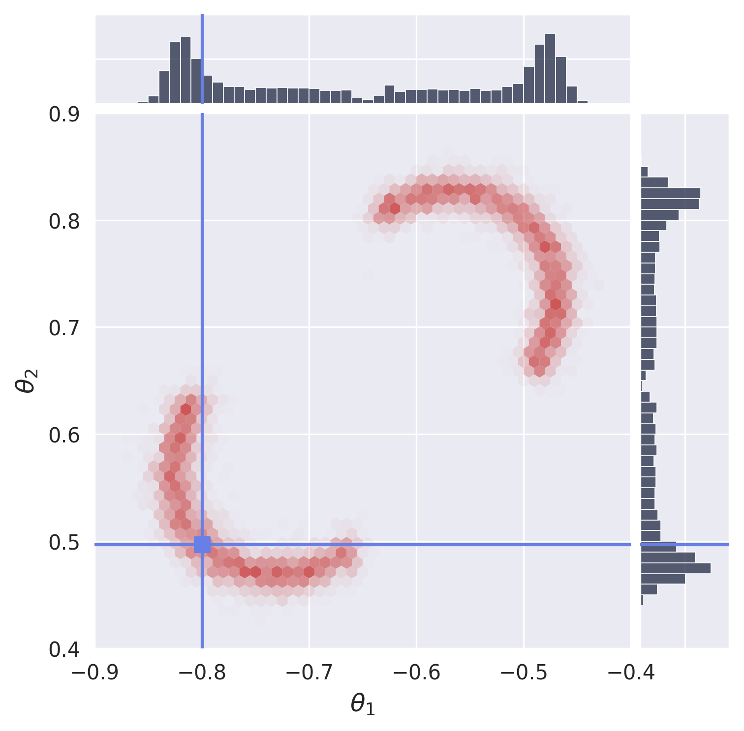
Cross-check. Tempered SMC and nested sampling estimate the same log-evidence \(\log p(x_o)\), so their two estimates are a mutual sanity check — for this observation they land within about \(0.1\) nat of each other (SMC \(\approx -0.70\), NS \(\approx -0.57 \pm 0.05\)). More importantly, two very different samplers recover the same two-crescent posterior, which is strong evidence that the learned MAF likelihood — and the multimodal sampling on top of it — are both behaving correctly.

The exact configuration used to train this checkpoint is in config/config_maf_nle.yaml. The full training + sampling script (which also writes these figures and a diagnostics file) is train_maf_nle.py.